Linear Mixed Models (LMMs)
Running linear mixed models to investigate the relationship between a predictor and a target over time using synthetic data intended to mimic the vitarenal data
Power calculation (based on repeated measures ANOVA, N=24, 4 time levels, and 2 equal sized groups, with 80% power and 5% alpha) shows that effects at the higher boundary of small effect sizes and the lower boundary of medium sized effects of Cohen’s d=.50-.55 (ƞ2=.07) can be reliably detected. This calculation allows for the planned linear mixed-model within-between interaction analyses, described at par. 8.3. For the analyses of main effects on the main endpoint/primary outcome (decrease over time on both cognitive biases within whole sample) the power with a N=24 sample size is considerably larger. Previous studies from our team among healthy volunteers with fatigue complaints showed similar effect sizes after less intensive single-session CBM (Pieterse & Bode, 2018). As LMM analyses can account for missing values effectively, partial missingness of datapoints is allowed and does not necessarily affect this power calculation.
N = 24,
Repeated measures = 4
Groups = 2
[1]:
2 * 4 * 24
[1]:
192
[2]:
from pymer4 import Lmer, simulate_lmm
import numpy as np
import pandas as pd
import seaborn as sns
import matplotlib.pyplot as plt
from utils import diagnostic_plots
import session_info
[3]:
session_info.show(write_req_file=False)
[3]:
Click to view session information
-----
matplotlib          3.5.2
numpy               1.22.4
pandas              1.1.5
pymer4              0.7.7
seaborn             0.11.2
session_info        1.0.0
utils               NA
-----
Click to view modules imported as dependencies
PIL                         9.1.1
appnope                     0.1.2
asttokens                   NA
backcall                    0.2.0
beta_ufunc                  NA
binom_ufunc                 NA
cffi                        1.15.0
cycler                      0.10.0
cython_runtime              NA
dateutil                    2.8.2
debugpy                     1.5.1
decorator                   5.1.1
deepdish                    0.3.7
defusedxml                  0.7.1
entrypoints                 0.4
executing                   0.8.3
hypergeom_ufunc             NA
ipykernel                   6.9.1
ipython_genutils            0.2.0
jedi                        0.18.1
jinja2                      3.1.2
joblib                      1.1.0
kiwisolver                  1.4.3
markupsafe                  2.1.1
mpl_toolkits                NA
nbinom_ufunc                NA
numexpr                     2.8.0
packaging                   21.3
parso                       0.8.3
patsy                       0.5.2
pexpect                     4.8.0
pickleshare                 0.7.5
pkg_resources               NA
prompt_toolkit              3.0.20
ptyprocess                  0.7.0
pure_eval                   0.2.2
pydev_ipython               NA
pydevconsole                NA
pydevd                      2.6.0
pydevd_concurrency_analyser NA
pydevd_file_utils           NA
pydevd_plugins              NA
pydevd_tracing              NA
pygments                    2.11.2
pyparsing                   3.0.9
pytz                        2022.1
pytz_deprecation_shim       NA
rpy2                        3.4.5
scipy                       1.8.1
setuptools                  59.8.0
six                         1.16.0
stack_data                  0.2.0
statsmodels                 0.13.2
tables                      3.7.0
tornado                     6.1
traitlets                   5.1.1
typing_extensions           NA
tzlocal                     NA
wcwidth                     0.2.5
zmq                         22.3.0
zoneinfo                    NA
-----
IPython             8.2.0
jupyter_client      7.2.2
jupyter_core        4.9.2
notebook            6.4.8
-----
Python 3.9.13 | packaged by conda-forge | (main, May 27 2022, 17:01:00) [Clang 13.0.1 ]
macOS-12.4-x86_64-i386-64bit
-----
Session information updated at 2022-06-28 21:35
[4]:
if "jms_style_sheet" in plt.style.available:
    plt.style.use("jms_style_sheet")
[5]:
number_observations = 4 # amount of observations per group (i.e. user_id)
number_predictors = 5
number_groups = 30 # amount of groups (i.e. user_id)

df, blups, coefficient = simulate_lmm(num_obs=number_observations,
    num_coef=number_predictors,
    num_grps=number_groups,
    coef_vals=None,
    corrs=None,
    grp_sigmas=0.25,
    mus=0.0,
    sigmas=1.0,
    noise_params=(0, 2),
    family='gaussian',
    seed=69420)

df = (df.assign(m00_name= lambda x: np.tile(["m00", "m03", "m06", "m09"], number_groups))
      .assign(diagnosis = np.repeat([0, 1], int(df.shape[0]/2)))
      .rename(columns={"Group": "user_id"}, inplace=False)
      .assign(user_id=lambda x: x["user_id"].astype(int))
      )
[6]:
display(df.head()), df.shape
| DV | IV1 | IV2 | IV3 | IV4 | IV5 | user_id | m00_name | diagnosis | |
|---|---|---|---|---|---|---|---|---|---|
| 0 | 1.310004 | 1.282629 | 0.041641 | 0.026445 | 1.112682 | -1.396378 | 1 | m00 | 0 |
| 1 | 0.348110 | -0.384780 | 0.663529 | -1.125871 | 0.127171 | 0.029313 | 1 | m03 | 0 |
| 2 | -0.901572 | -0.012763 | 0.031757 | 0.363677 | -1.443745 | -1.150963 | 1 | m06 | 0 |
| 3 | 1.684844 | -0.719206 | 0.488108 | 1.113077 | -0.524331 | 0.438103 | 1 | m09 | 0 |
| 4 | 0.840559 | 0.621639 | -1.237202 | 0.283866 | 1.043195 | -0.263725 | 2 | m00 | 0 |
[6]:
(None, (120, 9))
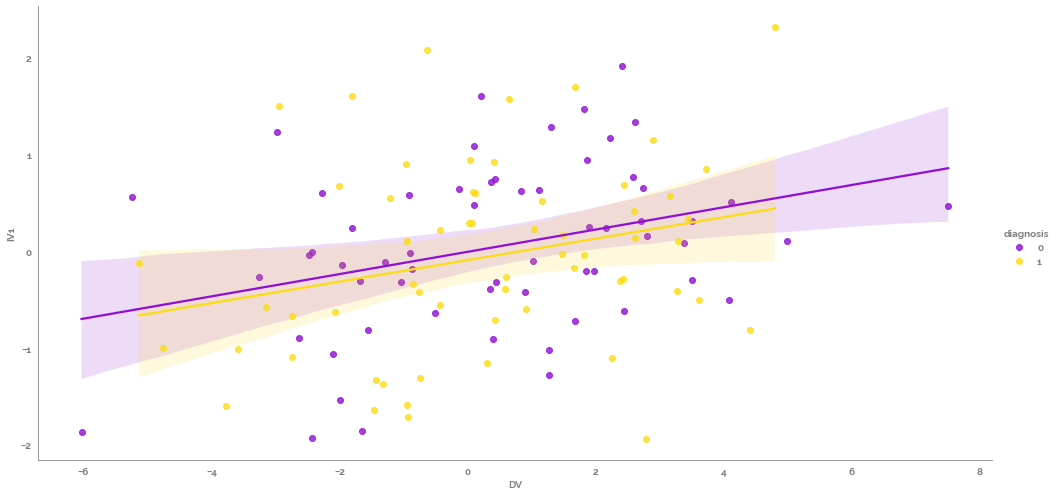
[7]:
_ = sns.lmplot(data=df, x="DV", y="IV1", hue="diagnosis", height=7, aspect=2)
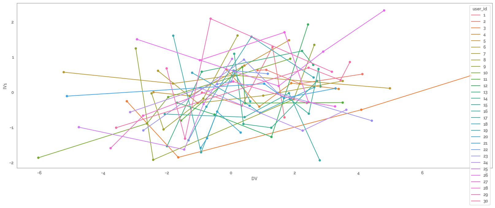
[8]:
_ = plt.figure(figsize=(20, 7))
_ = sns.lineplot(data=df.assign(user_id=lambda x: x["user_id"].astype("category")), x="DV", y="IV1", hue="user_id")
_ = sns.scatterplot(data=df.assign(user_id=lambda x: x["user_id"].astype("category")), x="DV", y="IV1", hue="user_id", legend=False)
Specify the predictor list
[9]:
predictor_list = df.filter(regex="IV").columns.tolist()

# df[predictor_list] = df[predictor_list].mask(np.random.random(df[predictor_list].shape) < .025)

dataLMM = df.dropna()
dataLMM.shape
[9]:
(120, 9)
[10]:
feature_collection = " + ".join(predictor_list[-2:4])
feature_collection
[10]:
'IV4'
Specify the model with the formula_string as the model syntax
[11]:
target_name = "DV"
[12]:
# formula_string = f"{target_name} ~ {feature_collection} + (1 + m00_name|user_id) + (1|diagnosis)"
formula_string = f"{target_name} ~ {feature_collection} + (1|user_id) + (1|m00_name) + (1|diagnosis)"
# formula_string = f"{target_name} ~ {feature_collection} + (1|diagnosis)"
print(formula_string)

model = Lmer(data=dataLMM, formula=formula_string)
DV ~ IV4 + (1|user_id) + (1|m00_name) + (1|diagnosis)
[13]:
# dataLMM.info()
Fit the model
Here you can specify factor levels of categorical features, and what approach you want used for confidence intervals of the coefficients
[14]:
# fixed_effect_output = model.fit(no_warnings=True, conf_int='profile') #model where the m00_name is not considered an ordered categorical feature
fixed_effect_output = model.fit(factors = {"m00_name": dataLMM["m00_name"].unique().tolist()},
                                ordered=True, no_warnings=True, conf_int='profile')

fixed_effect_output
Formula: DV~IV4+(1|user_id)+(1|m00_name)+(1|diagnosis)

Family: gaussian         Inference: parametric

Number of observations: 120      Groups: {'user_id': 30.0, 'm00_name': 4.0, 'diagnosis': 2.0}

Log-likelihood: -270.541         AIC: 541.081

Random effects:

                  Name    Var    Std
user_id    (Intercept)  0.000  0.000
m00_name   (Intercept)  0.000  0.000
diagnosis  (Intercept)  0.000  0.000
Residual                5.295  2.301

No random effect correlations specified

Fixed effects:
[14]:
| Estimate | 2.5_ci | 97.5_ci | SE | DF | T-stat | P-val | Sig | |
|---|---|---|---|---|---|---|---|---|
| (Intercept) | 0.305 | -0.168 | 0.778 | 0.211 | 118.0 | 1.446 | 0.151 | |
| IV4 | 0.720 | 0.298 | 1.141 | 0.215 | 118.0 | 3.346 | 0.001 | ** |
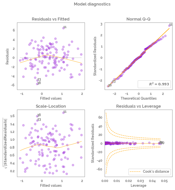
[15]:
fig, axs = diagnostic_plots(model_fit=model,
                                         X=None,
                                         y=None,
                                         figsize = (8,8),
                                         limit_cooks_plot = False,
                                         subplot_adjust_args={"wspace": 0.3, "hspace": 0.3}
                                        )