Mixed Effects Random Forests (MERF)
Running mixed effects random forests (MERF) to investigate the relationship between a predictor and a target over time using synthetic data intended to mimic the vitarenal data
Power calculation (based on repeated measures ANOVA, N=24, 4 time levels, and 2 equal sized groups, with 80% power and 5% alpha) shows that effects at the higher boundary of small effect sizes and the lower boundary of medium sized effects of Cohen’s d=.50-.55 (ƞ2=.07) can be reliably detected. This calculation allows for the planned linear mixed-model within-between interaction analyses, described at par. 8.3. For the analyses of main effects on the main endpoint/primary outcome (decrease over time on both cognitive biases within whole sample) the power with a N=24 sample size is considerably larger. Previous studies from our team among healthy volunteers with fatigue complaints showed similar effect sizes after less intensive single-session CBM (Pieterse & Bode, 2018). As LMM analyses can account for missing values effectively, partial missingness of datapoints is allowed and does not necessarily affect this power calculation.
N = 24,
Repeated measures = 4
Groups = 2
[1]:
2 * 4 * 24
[1]:
192
[2]:
from pymer4 import Lmer, simulate_lmm
import numpy as np
import pandas as pd
import seaborn as sns
import matplotlib.pyplot as plt
from local_MERF import MERF
# from jmspack.ml_utils import optimize_model
# from jmspack.utils import silence_stdout
from sklearn.ensemble import RandomForestRegressor
from sklearn.metrics import mean_squared_error
from matplotlib.lines import Line2D
import session_info
import pingouin as pg
[3]:
session_info.show(write_req_file=False)
[3]:
Click to view session information
-----
local_MERF          NA
matplotlib          3.5.2
numpy               1.22.4
pandas              1.1.5
pingouin            0.5.2
pymer4              0.7.7
seaborn             0.11.2
session_info        1.0.0
sklearn             1.0.2
-----
Click to view modules imported as dependencies
PIL                         9.1.1
appnope                     0.1.2
asttokens                   NA
backcall                    0.2.0
beta_ufunc                  NA
binom_ufunc                 NA
brotli                      NA
certifi                     2022.06.15
cffi                        1.15.0
charset_normalizer          2.0.4
cycler                      0.10.0
cython_runtime              NA
dateutil                    2.8.2
debugpy                     1.5.1
decorator                   5.1.1
deepdish                    0.3.7
defusedxml                  0.7.1
entrypoints                 0.4
executing                   0.8.3
hypergeom_ufunc             NA
idna                        3.3
ipykernel                   6.9.1
ipython_genutils            0.2.0
jedi                        0.18.1
jinja2                      3.1.2
joblib                      1.1.0
kiwisolver                  1.4.3
littleutils                 NA
markupsafe                  2.1.1
mpl_toolkits                NA
nbinom_ufunc                NA
numexpr                     2.8.0
outdated                    0.2.1
packaging                   21.3
pandas_flavor               NA
parso                       0.8.3
patsy                       0.5.2
pexpect                     4.8.0
pickleshare                 0.7.5
pkg_resources               NA
prompt_toolkit              3.0.20
ptyprocess                  0.7.0
pure_eval                   0.2.2
pydev_ipython               NA
pydevconsole                NA
pydevd                      2.6.0
pydevd_concurrency_analyser NA
pydevd_file_utils           NA
pydevd_plugins              NA
pydevd_tracing              NA
pygments                    2.11.2
pyparsing                   3.0.9
pytz                        2022.1
pytz_deprecation_shim       NA
requests                    2.27.1
rpy2                        3.4.5
scipy                       1.8.1
setuptools                  59.8.0
six                         1.16.0
socks                       1.7.1
stack_data                  0.2.0
statsmodels                 0.13.2
tables                      3.7.0
tabulate                    0.8.9
threadpoolctl               2.2.0
tornado                     6.1
traitlets                   5.1.1
typing_extensions           NA
tzlocal                     NA
unicodedata2                NA
urllib3                     1.26.9
wcwidth                     0.2.5
xarray                      0.20.1
zmq                         22.3.0
zoneinfo                    NA
-----
IPython             8.2.0
jupyter_client      7.2.2
jupyter_core        4.9.2
notebook            6.4.8
-----
Python 3.9.13 | packaged by conda-forge | (main, May 27 2022, 17:01:00) [Clang 13.0.1 ]
macOS-12.4-x86_64-i386-64bit
-----
Session information updated at 2022-06-28 21:36
[4]:
if "jms_style_sheet" in plt.style.available:
    plt.style.use("jms_style_sheet")
[5]:
number_observations = 4 # amount of observations per group (i.e. user_id)
number_predictors = 5
number_groups = 40 # amount of groups (i.e. user_id)

df, blups, coefficient = simulate_lmm(num_obs=number_observations,
    num_coef=number_predictors,
    num_grps=number_groups,
    coef_vals=None,
    corrs=None,
    grp_sigmas=0.25,
    mus=0.0,
    sigmas=1.0,
    noise_params=(0, 2),
    family='gaussian',
    seed=69420)

df = (df.assign(m00_name= lambda x: np.tile(["m00", "m03", "m06", "m09"], number_groups))
      .assign(diagnosis = np.repeat([0, 1], int(df.shape[0]/2)))
      .rename(columns={"Group": "user_id"}, inplace=False)
      .assign(user_id=lambda x: x["user_id"].astype(int))
      )
[6]:
coefficient
[6]:
array([0.53109224, 0.35676397, 0.51311614, 0.32530468, 0.45724967,
       0.01407327])
[7]:
display(df.head()), df.shape
| DV | IV1 | IV2 | IV3 | IV4 | IV5 | user_id | m00_name | diagnosis | |
|---|---|---|---|---|---|---|---|---|---|
| 0 | -0.176284 | -0.631297 | -1.545416 | 0.551350 | 0.465951 | 1.825298 | 1 | m00 | 0 |
| 1 | 5.297406 | -0.953989 | 1.068107 | -0.375538 | -0.775013 | 1.870303 | 1 | m03 | 0 |
| 2 | 1.694839 | -1.404839 | 2.835310 | -0.413594 | -1.253913 | -1.061551 | 1 | m06 | 0 |
| 3 | 2.079718 | -0.369729 | -0.014778 | 0.255887 | -0.590729 | 0.608351 | 1 | m09 | 0 |
| 4 | 3.061051 | 0.047046 | 0.517653 | 1.551487 | 0.089594 | 1.478871 | 2 | m00 | 0 |
[7]:
(None, (160, 9))
[8]:
predictor_list = df.filter(regex="IV").columns.tolist()[-2:4]

# df[predictor_list] = df[predictor_list].mask(np.random.random(df[predictor_list].shape) < .025)
[9]:
target = "DV"
grp = "user_id"
[10]:
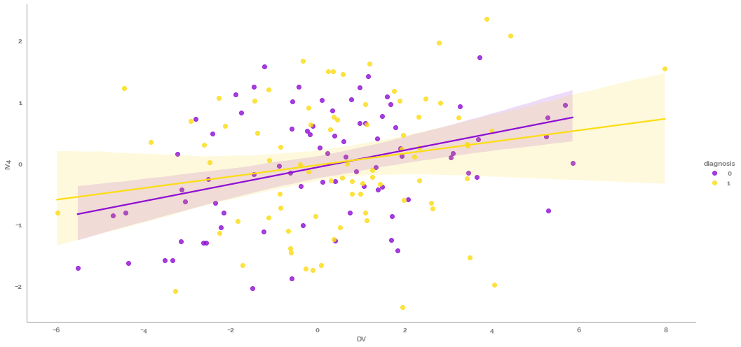
_ = sns.lmplot(data=df, x=target, y=predictor_list[0], hue="diagnosis", height=7, aspect=2)
[11]:
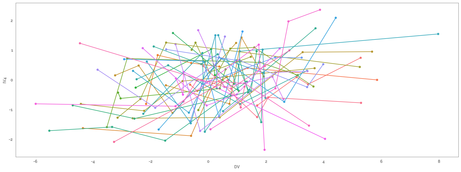
_ = plt.figure(figsize=(20, 7))
_ = sns.lineplot(data=df.assign(user_id=lambda x: x[grp].astype("category")), x=target, y=predictor_list[0], hue=grp, legend=False)
_ = sns.scatterplot(data=df.assign(user_id=lambda x: x[grp].astype("category")), x=target, y=predictor_list[0], hue=grp, legend=False)
[12]:
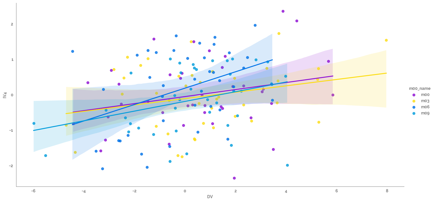
_ = sns.lmplot(data=df, x=target, y=predictor_list[0], hue="m00_name", height=7, aspect=2)
[13]:
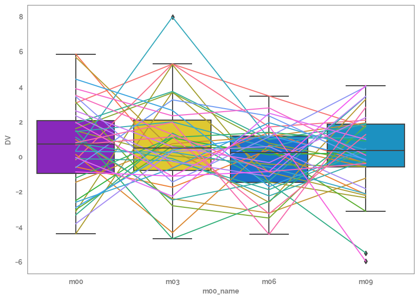
_ = plt.figure(figsize=(10, 7))
_ = sns.boxplot(data=df, x="m00_name", y=target)
_ = sns.lineplot(data=df.assign(user_id=lambda x: x[grp].astype("category")), x="m00_name", y=target, hue=grp, legend=False)
Specify the predictor list, target and group
Create train_test and hold out users
[14]:
hold_out_users = df.sample(n=5, random_state=69420)["user_id"].unique().tolist()
train_test_users = df[~df['user_id'].isin(hold_out_users)]["user_id"].unique().tolist()
[15]:
X = df.loc[df["user_id"].isin(train_test_users), predictor_list + [grp]]
y = df.loc[df["user_id"].isin(train_test_users), target]

hold_X = df.loc[df["user_id"].isin(hold_out_users), predictor_list + [grp]]
hold_y = df.loc[df["user_id"].isin(hold_out_users), target]
[16]:
X_train = X.sample(frac=0.8, random_state=42)
X_test = X.drop(X_train.index, axis=0)
y_train = y.loc[X_train.index]
y_test = y.drop(X_train.index, axis=0)
[17]:
print(X_train.shape); print(y_train.shape); print(X_test.shape); print(y_test.shape); print(hold_X.shape); print(hold_y.shape)
(112, 2)
(112,)
(28, 2)
(28,)
(20, 2)
(20,)
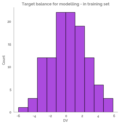
[18]:
_ = sns.displot(x=y_train, bins=10)
_ = plt.title("Target balance for modelling - in training set")
[19]:
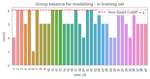
_ = plt.figure(figsize=(7,3))
_ = sns.countplot(x=X_train[grp])
_ = plt.title("Group balance for modelling - in training set")
cutoff = 4
_ = plt.axhline(cutoff, c="red",ls="--", label=f"Row Count Cutoff == {cutoff}")
_ = plt.legend()
_ = plt.xticks(rotation=90)
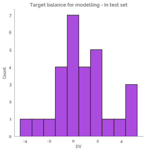
[20]:
# _ = plt.figure(figsize=(30,5))
_ = sns.displot(x=y_test, bins=10)
_ = plt.title("Target balance for modelling - in test set")
[21]:
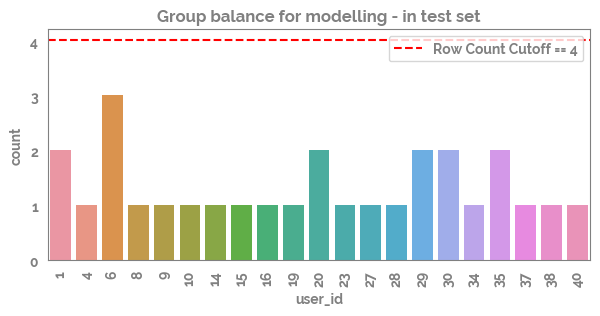
_ = plt.figure(figsize=(7,3))
_ = sns.countplot(x=X_test[grp])
_ = plt.title("Group balance for modelling - in test set")
cutoff = 4
_ = plt.axhline(cutoff, c="red", ls="--", label=f"Row Count Cutoff == {cutoff}")
_ = plt.legend()
_ = plt.xticks(rotation=90)
_ = plt.show()
[22]:
tmp = X_train.apply(lambda x: x.nunique()).sort_values()
tmp
[22]:
user_id     35
IV4        112
dtype: int64
[23]:
n_it = 100 # specify the maximum amount of iterations you would like the MERF to use during expectation–maximization (EM)
rf_params={"n_estimators": 300, "criterion": "squared_error", "max_features": "sqrt", "oob_score": True}
merf = MERF(n_estimators=300, gll_early_stop_threshold=0.001, max_iterations=n_it, rf_params=rf_params)
_ = merf.fit(X=X_train, Z=np.ones((len(X_train), 1)), clusters=X_train[grp], y=y_train)
y_pred = merf.predict(X=X_test, Z=np.ones((len(X_test), 1)), clusters=X_test[grp])
[24]:
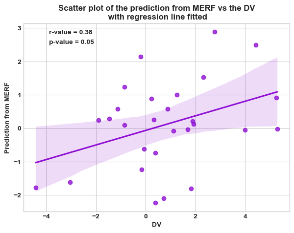
pred_test_df=pd.DataFrame({"y_pred": y_pred, target: y_test, 'user_id': X_test['user_id']})
# pred_test_df = pred_test_df.groupby('user_id').mean()
merf_cors = pg.corr(pred_test_df["y_pred"], pred_test_df[target])
merf_cors
[24]:
| n | r | CI95% | p-val | BF10 | power | |
|---|---|---|---|---|---|---|
| pearson | 28 | 0.378408 | [0.01, 0.66] | 0.047079 | 1.533 | 0.524503 |
[25]:
from matplotlib.lines import Line2D
plt.style.use('seaborn-whitegrid')
legend_elements = [Line2D([0], [0], marker="", color="k", label=f"r-value = {np.round(merf_cors['r'].iat[0],2)}", linestyle="none", ),
                  Line2D([0], [0], marker="", color="k", label=f"p-value = {np.round(merf_cors['p-val'].iat[0],2)}", linestyle="none", )]
fig, ax = plt.subplots(figsize=(7,5))
sns.regplot(x=target, y="y_pred", data=pred_test_df).\
set_title(f"Scatter plot of the prediction from MERF vs the {target}\n with regression line fitted")
_ = ax.legend(handles=legend_elements)
plt.xlabel(target)
plt.ylabel(f"Prediction from MERF")
plt.show()
[26]:
user_id_min=pred_test_df.index.min()
user_id_max=pred_test_df.index.max()
[27]:
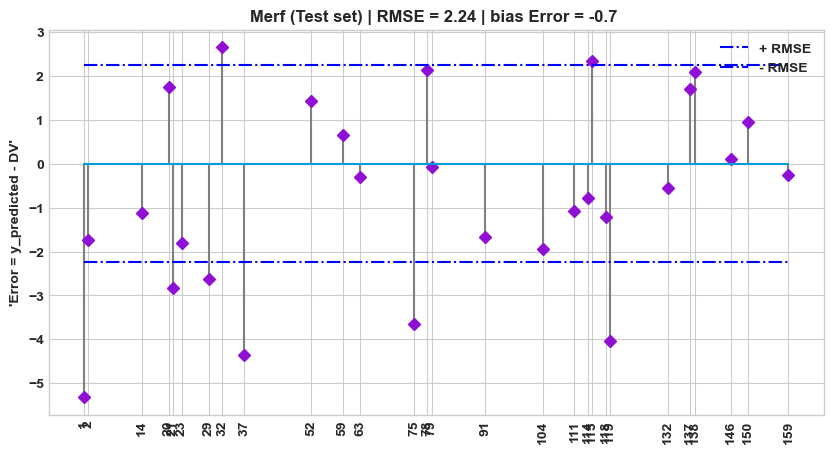
df_test=pred_test_df
# plt.style.use('ggplot')
plt.figure(figsize=(10,5))
plt.title(f"Merf (Test set) | RMSE = {round(np.sqrt(mean_squared_error(df_test['y_pred'], df_test[target])),2)} | bias Error = { round(np.mean(df_test['y_pred'] - df_test[target]), 2)} ")
plt.stem(df_test.index, df_test['y_pred'] - df_test[target], use_line_collection=True, linefmt='grey', markerfmt='D')
plt.hlines(y=round(np.sqrt(mean_squared_error(df_test['y_pred'], df_test[target])),2), colors='b', linestyles='-.', label='+ RMSE', xmin = user_id_min, xmax = user_id_max)
plt.hlines(y=round(-np.sqrt(mean_squared_error(df_test['y_pred'], df_test[target])),2), colors='b', linestyles='-.', label='- RMSE', xmin = user_id_min, xmax = user_id_max)
plt.xticks(rotation=90, ticks=df_test.index)
plt.ylabel(f"'Error = y_predicted - {target}'")
# plt.ylim([-.5,.6])
plt.legend()
_ = plt.show()
Hold out set
[28]:
y_pred = merf.predict(X=hold_X, Z=np.ones((len(hold_X), 1)), clusters=hold_X[grp])
[29]:
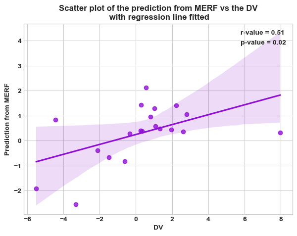
pred_test_df=pd.DataFrame({"y_pred": y_pred, target: hold_y, grp: hold_X[grp]})
# pred_test_df = pred_test_df.groupby(grp).mean()
merf_cors = pg.corr(pred_test_df["y_pred"], pred_test_df[target])
merf_cors
[29]:
| n | r | CI95% | p-val | BF10 | power | |
|---|---|---|---|---|---|---|
| pearson | 20 | 0.511412 | [0.09, 0.78] | 0.021181 | 3.31 | 0.661748 |
[30]:
plt.style.use('seaborn-whitegrid')
legend_elements = [Line2D([0], [0], marker="", color="k", label=f"r-value = {np.round(merf_cors['r'].iat[0],2)}", linestyle="none", ),
                  Line2D([0], [0], marker="", color="k", label=f"p-value = {np.round(merf_cors['p-val'].iat[0],2)}", linestyle="none", )]
fig, ax = plt.subplots(figsize=(7,5))
sns.regplot(x=target, y="y_pred", data=pred_test_df).\
set_title(f"Scatter plot of the prediction from MERF vs the {target}\n with regression line fitted")
_ = ax.legend(handles=legend_elements)
plt.xlabel(target)
plt.ylabel(f"Prediction from MERF")
plt.show()
[31]:
user_id_min=pred_test_df.index.min()
user_id_max=pred_test_df.index.max()
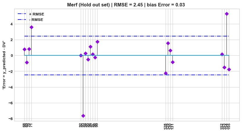
[32]:
df_test=pred_test_df
# plt.style.use('ggplot')
plt.figure(figsize=(10, 5))
plt.title(f"Merf (Hold out set) | RMSE = {round(np.sqrt(mean_squared_error(df_test['y_pred'], df_test[target])),2)} | bias Error = { round(np.mean(df_test['y_pred'] - df_test[target]), 2)} ")
plt.stem(df_test.index, df_test['y_pred'] - df_test[target], use_line_collection=True, linefmt='grey', markerfmt='D')
plt.hlines(y=round(np.sqrt(mean_squared_error(df_test['y_pred'], df_test[target])),2), colors='b', linestyles='-.', label='+ RMSE', xmin = user_id_min, xmax = user_id_max)
plt.hlines(y=round(-np.sqrt(mean_squared_error(df_test['y_pred'], df_test[target])),2), colors='b', linestyles='-.', label='- RMSE', xmin = user_id_min, xmax = user_id_max)
plt.xticks(rotation=90, ticks=df_test.index)
plt.ylabel(f"'Error = y_predicted - {target}'")
# plt.ylim([-.5,.6])
plt.legend()
_ = plt.show()