Sleep EMA Linear Mixed Models (LMM)
Replication Data for Wu et al. (2020) “Multi-Modal Data Collection for Measuring Health, Behavior, and Living Environment of Large-Scale Participant Cohorts: Conceptual Framework and Findings from Deployments”: Ecological Momentary Assessment Data (Beiwe)
[1]:
import pandas as pd
import numpy as np
from glob import glob
import seaborn as sns
import matplotlib.pyplot as plt
from pymer4 import Lmer
from helpers import diagnostic_plots
from jmspack.utils import JmsColors
[2]:
if "jms_style_sheet" in plt.style.available:
    plt.style.use("jms_style_sheet")
[3]:
df = (pd.read_csv("data/UT1000_ema_wide.csv")
      .dropna()
      .assign(**{"date": lambda d: pd.to_datetime(d["survey.date"])})
      # .pipe(lambda d: d[d["survey.date"].str.contains("2019")])
      .drop("survey.date", axis=1)
      .pipe(lambda d: d[d["date"] <= pd.to_datetime("03-15-2019")])
      .pipe(lambda d: d[d["date"] >= pd.to_datetime("02-14-2019")])
      .sort_values(["pid", "date"])
      .reset_index(drop=True)
      )
display(df.head()); df.shape
| pid | content | energy | lonely | refreshed | restful | sad | sleep | stress | date | |
|---|---|---|---|---|---|---|---|---|---|---|
| 0 | 1193rv5x | 3.0 | 3.0 | 2.0 | 2.0 | 3.0 | 1.0 | 5.0 | 1.0 | 2019-02-14 |
| 1 | 1193rv5x | 2.0 | 3.0 | 3.0 | 1.0 | 2.0 | 2.0 | 6.0 | 1.0 | 2019-02-15 |
| 2 | 1193rv5x | 1.0 | 2.0 | 3.0 | 1.0 | 2.0 | 2.0 | 9.0 | 1.0 | 2019-02-16 |
| 3 | 1193rv5x | 1.0 | 1.0 | 3.0 | 2.0 | 2.0 | 3.0 | 9.0 | 2.0 | 2019-02-17 |
| 4 | 1193rv5x | 3.0 | 3.0 | 1.0 | 1.0 | 2.0 | 1.0 | 5.0 | 1.0 | 2019-02-18 |
[3]:
(4913, 10)
[4]:
print(df.date.min()); print(df.date.max())
2019-02-14 00:00:00
2019-03-15 00:00:00
[5]:
df.info()
<class 'pandas.core.frame.DataFrame'>
RangeIndex: 4913 entries, 0 to 4912
Data columns (total 10 columns):
 #   Column     Non-Null Count  Dtype
---  ------     --------------  -----
 0   pid        4913 non-null   object
 1   content    4913 non-null   float64
 2   energy     4913 non-null   float64
 3   lonely     4913 non-null   float64
 4   refreshed  4913 non-null   float64
 5   restful    4913 non-null   float64
 6   sad        4913 non-null   float64
 7   sleep      4913 non-null   float64
 8   stress     4913 non-null   float64
 9   date       4913 non-null   datetime64[ns]
dtypes: datetime64[ns](1), float64(8), object(1)
memory usage: 384.0+ KB
[6]:
df.describe()
[6]:
| content | energy | lonely | refreshed | restful | sad | sleep | stress | |
|---|---|---|---|---|---|---|---|---|
| count | 4913.000000 | 4913.000000 | 4913.000000 | 4913.000000 | 4913.000000 | 4913.000000 | 4913.000000 | 4913.000000 |
| mean | 1.871565 | 2.134948 | 0.513332 | 1.618563 | 1.834724 | 0.591696 | 6.237737 | 1.175453 |
| std | 0.823113 | 0.830693 | 0.731918 | 0.881945 | 0.858564 | 0.773247 | 1.687056 | 0.882876 |
| min | 0.000000 | 0.000000 | 0.000000 | 0.000000 | 0.000000 | 0.000000 | 0.000000 | 0.000000 |
| 25% | 1.000000 | 2.000000 | 0.000000 | 1.000000 | 1.000000 | 0.000000 | 5.000000 | 1.000000 |
| 50% | 2.000000 | 2.000000 | 0.000000 | 2.000000 | 2.000000 | 0.000000 | 6.000000 | 1.000000 |
| 75% | 2.000000 | 3.000000 | 1.000000 | 2.000000 | 2.000000 | 1.000000 | 7.000000 | 2.000000 |
| max | 3.000000 | 4.000000 | 3.000000 | 3.000000 | 3.000000 | 3.000000 | 12.000000 | 3.000000 |
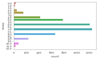
[7]:
target="sleep"
group="pid"
checkpoint="date"
feature_list=df.select_dtypes(float).drop(target, axis=1).columns.tolist()
_ = plt.figure(figsize=(5,3))
_ = sns.countplot(y=df[target])
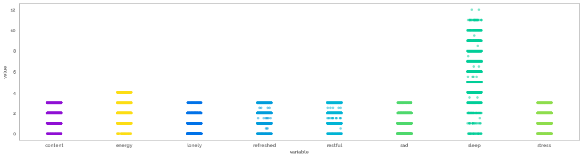
[8]:
_ = plt.figure(figsize=(20, 5))
_ = sns.stripplot(data=df.select_dtypes(float).melt(), x="variable", y="value", alpha=0.5)
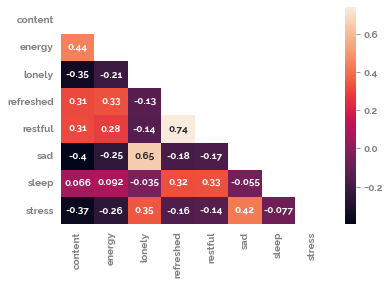
[9]:
mask = np.triu(np.ones_like(df.corr(), dtype=bool))
_ = sns.heatmap(df.corr(method="spearman"), mask=mask, annot=True)
[10]:
cluster_collection = "+".join(feature_list)
cluster_collection
[10]:
'content+energy+lonely+refreshed+restful+sad+stress'
[11]:
formula_string = f"{target} ~ {cluster_collection} + (1 | {group}) + (1 | {checkpoint})"
model = Lmer(data=df, formula=formula_string)
initial_mod_fixed_eff = model.fit(no_warnings=True)
initial_mod_fixed_eff
Formula: sleep~content+energy+lonely+refreshed+restful+sad+stress+(1|pid)+(1|date)

Family: gaussian         Inference: parametric

Number of observations: 4913     Groups: {'pid': 411.0, 'date': 30.0}

Log-likelihood: -8756.933        AIC: 17513.866

Random effects:

                 Name    Var    Std
pid       (Intercept)  0.710  0.843
date      (Intercept)  0.046  0.214
Residual               1.780  1.334

No random effect correlations specified

Fixed effects:
[11]:
| Estimate | 2.5_ci | 97.5_ci | SE | DF | T-stat | P-val | Sig | |
|---|---|---|---|---|---|---|---|---|
| (Intercept) | 4.929 | 4.690 | 5.169 | 0.122 | 1006.443 | 40.325 | 0.000 | *** |
| content | -0.064 | -0.135 | 0.007 | 0.036 | 4733.664 | -1.766 | 0.077 | . |
| energy | 0.025 | -0.035 | 0.085 | 0.031 | 4876.512 | 0.826 | 0.409 | |
| lonely | 0.026 | -0.059 | 0.110 | 0.043 | 4871.830 | 0.596 | 0.551 | |
| refreshed | 0.338 | 0.268 | 0.408 | 0.036 | 4755.562 | 9.434 | 0.000 | *** |
| restful | 0.433 | 0.361 | 0.505 | 0.037 | 4766.650 | 11.838 | 0.000 | *** |
| sad | 0.010 | -0.070 | 0.090 | 0.041 | 4878.341 | 0.237 | 0.813 | |
| stress | -0.040 | -0.099 | 0.019 | 0.030 | 4885.360 | -1.327 | 0.184 |
[12]:
cluster_collection="refreshed+restful"
formula_string = f"{target} ~ {cluster_collection} + (1 | {group}) + (1 | {checkpoint})"
model = Lmer(data=df, formula=formula_string)
fixed_eff = model.fit(no_warnings=True)
fixed_eff
Formula: sleep~refreshed+restful+(1|pid)+(1|date)

Family: gaussian         Inference: parametric

Number of observations: 4913     Groups: {'pid': 411.0, 'date': 30.0}

Log-likelihood: -8747.223        AIC: 17494.446

Random effects:

                 Name    Var    Std
pid       (Intercept)  0.714  0.845
date      (Intercept)  0.046  0.214
Residual               1.780  1.334

No random effect correlations specified

Fixed effects:
[12]:
| Estimate | 2.5_ci | 97.5_ci | SE | DF | T-stat | P-val | Sig | |
|---|---|---|---|---|---|---|---|---|
| (Intercept) | 4.840 | 4.685 | 4.996 | 0.079 | 228.722 | 61.103 | 0.0 | *** |
| refreshed | 0.339 | 0.270 | 0.409 | 0.035 | 4781.391 | 9.574 | 0.0 | *** |
| restful | 0.429 | 0.357 | 0.500 | 0.036 | 4786.763 | 11.765 | 0.0 | *** |
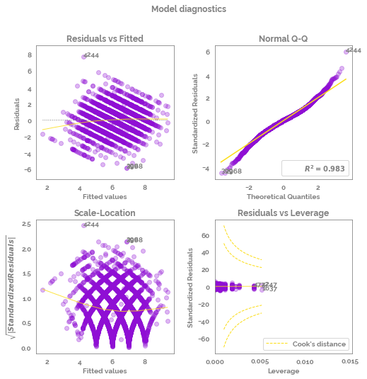
[13]:
try:
    fig, axs = diagnostic_plots(model_fit=model,
                                         X=None,
                                         y=None,
                                         figsize = (8,8),
                                         limit_cooks_plot = False,
                                         subplot_adjust_args={"wspace": 0.3, "hspace": 0.3}
                                        )
except:
    print("The function did not run - this is likely due to multiple random effects being specified")
[14]:
def r2_GLMM(model):
    sigma2_fe = model.design_matrix.multiply(model.fixef[0].mean()).var().sum()
    sigma2_re = model.ranef_var.loc[group, "Var"]
    sigma2_ol = model.ranef_var.loc["Residual", "Var"]
    r2_marginal = (sigma2_fe) / (sigma2_fe + sigma2_re + sigma2_ol)
    r2_conditional = (sigma2_fe + sigma2_re) / (sigma2_fe + sigma2_re + sigma2_ol)

    return pd.DataFrame({"Marginal_R_squared": r2_marginal,
                        "Conditional_R_squared": r2_conditional},
                       index=[0])
Conditional and marginal R squared
based on Nakagawa, S., & Schielzeth, H. (2013). A general and simple method for obtaining R2 from generalized linear mixed‐effects models. Methods in ecology and evolution, 4(2), 133-142.
Marginal R-squared is the R-squared for just the fixed effects
Conditional R-squared is the R-squared for both the fixed effects and random effects
[15]:
r2_GLMM(model)
[15]:
| Marginal_R_squared | Conditional_R_squared | |
|---|---|---|
| 0 | 0.082767 | 0.34553 |
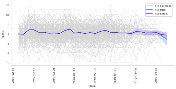
[16]:
predict_df = df.assign(**{f"{target}_fitted": model.fits})
[19]:
_ = plt.figure(figsize=(10, 4))
ax = sns.lineplot(data=predict_df,
                 x=checkpoint,
                 y=target,
                 hue=group,
                 palette=list(np.repeat(JmsColors.OFFWHITE, repeats=predict_df[group].nunique())),
                 legend=False,
                 alpha=0.4)
_ = sns.lineplot(data=predict_df,
                 x=checkpoint,
                 y=target,
                 color=JmsColors.DARKBLUE,
                 ax=ax)
_ = sns.lineplot(data=predict_df,
                 x=checkpoint,
                 y=f"{target}_fitted",
                 color=JmsColors.PURPLE,
                 ax=ax)
_ = plt.xticks(rotation=90)
_ = plt.plot([], [], label=f"{group} per user", c=JmsColors.OFFWHITE)
_ = plt.plot([], [], label=f"{group} true", c=JmsColors.DARKBLUE)
_ = plt.plot([], [], label=f"{group} fitted", c=JmsColors.PURPLE)
_ = plt.legend()
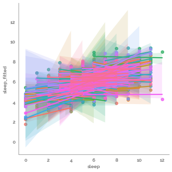
[18]:
_ = sns.lmplot(data=predict_df, x=target, y=f"{target}_fitted", hue=group, legend=False)