PIMA diabetes Classification
[1]:
import pandas as pd
import numpy as np
import matplotlib.pyplot as plt
import seaborn as sns
import session_info

from jmspack.utils import (apply_scaling,
                           JmsColors
                          )

from ml_class import (plot_cv_indices,
                      plot_decision_boundary,
                     plot_learning_curve,
                     multi_roc_auc_plot,
                     dict_of_models,
                     RFE_opt_rf,
                     make_confusion_matrix)

from sklearn.tree import DecisionTreeClassifier
from sklearn.linear_model import LogisticRegression
from sklearn.ensemble import (RandomForestClassifier,
                              GradientBoostingClassifier)
from sklearn.model_selection import (GridSearchCV,
                                     RepeatedStratifiedKFold,
                                     cross_val_score,
                                     cross_validate,
                                     train_test_split,
                                     KFold)
from sklearn.feature_selection import RFE
from sklearn.metrics import (confusion_matrix,
                             roc_curve,
                             auc)
from imblearn.over_sampling import (SMOTE,
                                    SVMSMOTE,
                                   KMeansSMOTE)
import shap
[2]:
# init the JS visualization code
shap.initjs()

[3]:
session_info.show(req_file_name="pima-requirements.txt",
      write_req_file=False) #add write_req_file=True to function to get requirements.txt file of packages used
[3]:
Click to view session information
-----
imblearn            0.8.1
jmspack             0.1.0
matplotlib          3.4.3
ml_class            NA
numpy               1.21.4
pandas              1.3.4
seaborn             0.11.2
session_info        1.0.0
shap                0.40.0
sklearn             1.0.1
-----
Click to view modules imported as dependencies
PIL                         8.4.0
anyio                       NA
appnope                     0.1.2
attr                        21.2.0
babel                       2.9.1
backcall                    0.2.0
beta_ufunc                  NA
binom_ufunc                 NA
brotli                      NA
certifi                     2021.10.08
cffi                        1.15.0
chardet                     4.0.0
charset_normalizer          2.0.0
cloudpickle                 2.0.0
colorama                    0.4.4
cycler                      0.10.0
cython_runtime              NA
dateutil                    2.8.2
debugpy                     1.5.1
decorator                   5.1.0
defusedxml                  0.7.1
entrypoints                 0.3
idna                        3.1
importlib_resources         NA
ipykernel                   6.5.0
ipython_genutils            0.2.0
jedi                        0.18.0
jinja2                      3.0.3
joblib                      1.1.0
json5                       NA
jsonschema                  4.2.1
jupyter_server              1.11.2
jupyterlab_server           2.8.2
kiwisolver                  1.3.2
llvmlite                    0.36.0
markupsafe                  2.0.1
matplotlib_inline           NA
mpl_toolkits                NA
nbclassic                   NA
nbformat                    5.1.3
nbinom_ufunc                NA
numba                       0.53.1
packaging                   21.0
parso                       0.8.2
pexpect                     4.8.0
pickleshare                 0.7.5
pkg_resources               NA
prometheus_client           NA
prompt_toolkit              3.0.22
ptyprocess                  0.7.0
pvectorc                    NA
pydev_ipython               NA
pydevconsole                NA
pydevd                      2.6.0
pydevd_concurrency_analyser NA
pydevd_file_utils           NA
pydevd_plugins              NA
pydevd_tracing              NA
pygments                    2.10.0
pyparsing                   3.0.6
pyrsistent                  NA
pytz                        2021.3
requests                    2.26.0
scipy                       1.7.2
send2trash                  NA
six                         1.16.0
slicer                      NA
sniffio                     1.2.0
socks                       1.7.1
statsmodels                 0.13.1
storemagic                  NA
terminado                   0.12.1
threadpoolctl               3.0.0
tornado                     6.1
tqdm                        4.62.3
traitlets                   5.1.1
urllib3                     1.26.7
wcwidth                     0.2.5
websocket                   0.57.0
zipp                        NA
zmq                         22.3.0
-----
IPython             7.29.0
jupyter_client      7.0.6
jupyter_core        4.9.1
jupyterlab          3.2.3
notebook            6.4.5
-----
Python 3.8.12 | packaged by conda-forge | (default, Oct 12 2021, 21:50:38) [Clang 11.1.0 ]
macOS-10.15.7-x86_64-i386-64bit
-----
Session information updated at 2021-11-14 19:59
[4]:
if "jms_style_sheet" in plt.style.available:
    plt.style.use("jms_style_sheet")
[5]:
df = pd.read_csv("diabetes.csv")
[6]:
display(df.head()), display(df.shape)
| Pregnancies | Glucose | BloodPressure | SkinThickness | Insulin | BMI | DiabetesPedigreeFunction | Age | Outcome | |
|---|---|---|---|---|---|---|---|---|---|
| 0 | 6 | 148 | 72 | 35 | 0 | 33.6 | 0.627 | 50 | 1 |
| 1 | 1 | 85 | 66 | 29 | 0 | 26.6 | 0.351 | 31 | 0 |
| 2 | 8 | 183 | 64 | 0 | 0 | 23.3 | 0.672 | 32 | 1 |
| 3 | 1 | 89 | 66 | 23 | 94 | 28.1 | 0.167 | 21 | 0 |
| 4 | 0 | 137 | 40 | 35 | 168 | 43.1 | 2.288 | 33 | 1 |
(768, 9)
[6]:
(None, None)
[7]:
target = "Outcome"
Mask 0 default values (seen in EDA)
[8]:
mask_default_values=True
[9]:
if mask_default_values:
    df = (df.drop([target, "Pregnancies"], axis=1)
           .replace(0, np.nan)
           .merge(df[[target, "Pregnancies"]], left_index=True, right_index=True)
          .dropna()
          .reset_index(drop=True)
         )
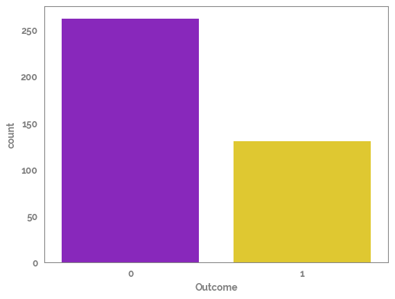
Plot the amount of rows in each side of the target
Looks like the target is imbalanced so this needs to be taken into account
[10]:
_ = sns.countplot(x=df[target])
print("Amount in each outcome")
df[target].value_counts()
Amount in each outcome
[10]:
0    262
1    130
Name: Outcome, dtype: int64
Resample data to correct for imbalance
[11]:
resample_data=True
[12]:
if resample_data:

    X = df.drop(target, axis=1)
    y = df[target]

    sm = KMeansSMOTE(sampling_strategy="not majority",
               random_state=42,
               n_jobs=2)
    X_res, y_res = sm.fit_resample(X, y)

    print(X.shape, y.shape, X_res.shape, y_res.shape)

    df = pd.concat([X_res, y_res], axis=1)
(392, 8) (392,) (525, 8) (525,)
[13]:
X = df.drop(target, axis=1)
y = df[target]
[14]:
dict_of_models
[14]:
[{'label': 'Logistic Regression', 'model': LogisticRegression()},
 {'label': 'Gradient Boosting', 'model': GradientBoostingClassifier()},
 {'label': 'K_Neighbors Classifier',
  'model': KNeighborsClassifier(n_neighbors=3)},
 {'label': 'SVM Classifier (linear)',
  'model': SVC(C=0.025, kernel='linear', probability=True)},
 {'label': 'SVM Classifier (Radial Basis Function; RBF)',
  'model': SVC(C=1, gamma=2, probability=True)},
 {'label': 'Gaussian Process Classifier',
  'model': GaussianProcessClassifier(kernel=1**2 * RBF(length_scale=1))},
 {'label': 'Decision Tree (depth=5)',
  'model': DecisionTreeClassifier(max_depth=5)},
 {'label': 'Random Forest Classifier(depth=5)',
  'model': RandomForestClassifier(max_depth=5, max_features=1, n_estimators=10)},
 {'label': 'Multilayer Perceptron (MLP) Classifier',
  'model': MLPClassifier(alpha=1, max_iter=1000)},
 {'label': 'AdaBoost Classifier', 'model': AdaBoostClassifier()},
 {'label': 'Naive Bayes (Gaussian) Classifier', 'model': GaussianNB()},
 {'label': 'Quadratic Discriminant Analysis Classifier',
  'model': QuadraticDiscriminantAnalysis()}]
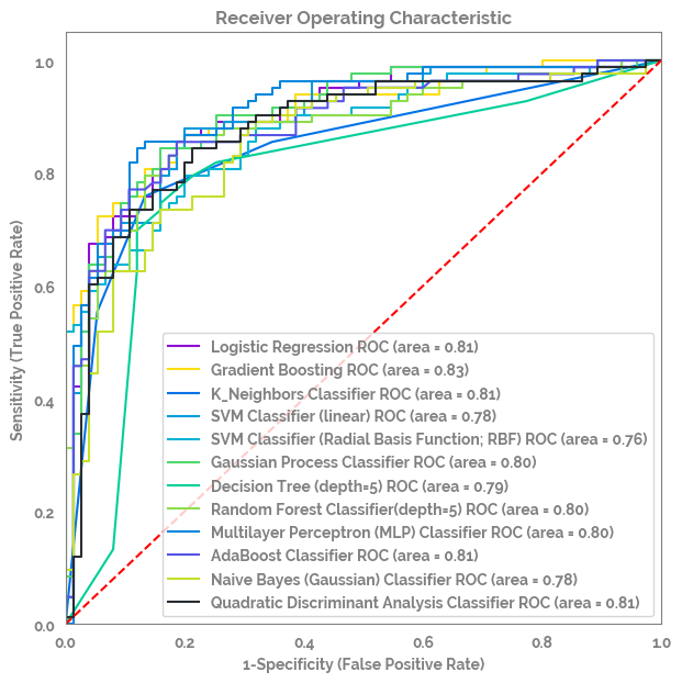
[15]:
_ = multi_roc_auc_plot(X=X,
                       y=y,
                       models=dict_of_models)
[16]:
n_features_to_select = 2 #[1, 2, 5, 10, 50, 100]
max_depth = [1, 2, 5, 10, 50, 100]
n_estimators = [1, 2, 5, 10, 50, 100, 120, 140, 160, 180, 200, 220, 240, 260, 280, 300]
[17]:
# Instanciate Random Forest
# rf = RandomForestClassifier(random_state = 42,
#                             oob_score    = False) # use oob_score with many trees

rf = GradientBoostingClassifier(random_state = 42)

# Define params_dt
params_rf = {'max_depth'    : max_depth,
#              'n_estimators' : n_estimators,
         'max_features' : ['log2', 'auto', 'sqrt'],
#          'criterion'    : ['gini', 'entropy'], #for RandomForestClassifier
           'criterion'    : ['friedman_mse', 'squared_error'] #for GradientBoostingClassifier
            }

# Instantiate grid_dt
grid_dt = GridSearchCV(estimator  = rf,
                   param_grid = params_rf,
                   scoring    = 'roc_auc',
                   cv         = 3,
                   n_jobs     = -2)

# Optimize hyperparameter
_ = grid_dt.fit(X, y)

# Extract the best estimator
optimized_rf = grid_dt.best_estimator_

# Create the RFE with a optimized random forest
# rfe = RFE(estimator            = optimized_rf,
#           n_features_to_select = n_features_to_select,
#           verbose              = 1)

rfe = RFE(estimator            = optimized_rf,
      n_features_to_select = n_features_to_select,
      verbose              = 1)

# Fit the eliminator to the data
_ = rfe.fit(X, y)

# create dataframe with features ranking (high = dropped early on)
feature_ranking = pd.DataFrame(data  = dict(zip(X.columns, rfe.ranking_)) ,
                           index = np.arange(0, len(X.columns)))
feature_ranking = feature_ranking.loc[0,:].sort_values()

# create dataframe with feature selected
feature_selected = X.columns[rfe.support_].to_list()

# create dataframe with importances per feature
feature_importance = pd.Series(dict(zip(X.columns, optimized_rf.feature_importances_.round(2))))

max_depth = optimized_rf.get_params()['max_depth']
max_features = optimized_rf.get_params()['max_features']
criterion = optimized_rf.get_params()['criterion']
Fitting estimator with 8 features.
Fitting estimator with 7 features.
Fitting estimator with 6 features.
Fitting estimator with 5 features.
Fitting estimator with 4 features.
Fitting estimator with 3 features.
[18]:
feature_importance_df = pd.DataFrame(feature_importance.sort_values(ascending=False)).reset_index().rename(columns={"index": "feature", 0: "feature_importance"})
[19]:
criterion, max_features, max_depth
[19]:
('friedman_mse', 'sqrt', 5)
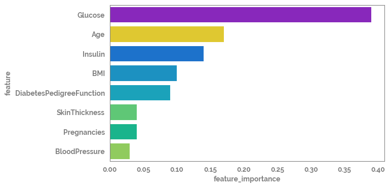
[20]:
feature_importance_df
[20]:
| feature | feature_importance | |
|---|---|---|
| 0 | Glucose | 0.39 |
| 1 | Age | 0.17 |
| 2 | Insulin | 0.14 |
| 3 | BMI | 0.10 |
| 4 | DiabetesPedigreeFunction | 0.09 |
| 5 | SkinThickness | 0.04 |
| 6 | Pregnancies | 0.04 |
| 7 | BloodPressure | 0.03 |
[21]:
_ = plt.figure(figsize=(7, 4))
_ = sns.barplot(data=feature_importance_df, x="feature_importance", y="feature")
# _ = plt.savefig("images/feature_importances_diabetes_all.png", dpi=400, bbox_inches="tight")
[22]:
explainer = shap.Explainer(optimized_rf)
shap_values = explainer(X)
[23]:
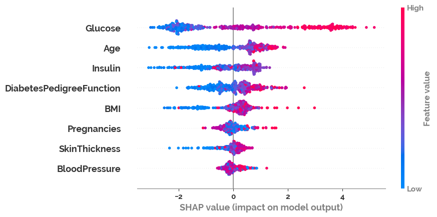
shap.plots.beeswarm(shap_values)
[24]:
clf = optimized_rf
kfold = KFold(n_splits=5, shuffle=True, random_state=1)
# enumerate the splits and summarize the distributions
for train_ix, test_ix in kfold.split(X):
# select rows
train_X, test_X = X.loc[train_ix, :], X.loc[test_ix, :]
train_y, test_y = y.loc[train_ix], y.loc[test_ix]
# summarize train and test composition
train_0, train_1 = len(train_y[train_y==0]), len(train_y[train_y==1])
test_0, test_1 = len(test_y[test_y==0]), len(test_y[test_y==1])
print('>Train: 0=%d, 1=%d, Test: 0=%d, 1=%d' % (train_0, train_1, test_0, test_1))
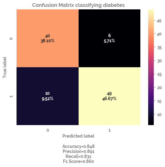
_ = clf.fit(X = train_X,
y = train_y)
pred_y = clf.predict(test_X)
cf_matrix = confusion_matrix(test_y, pred_y)
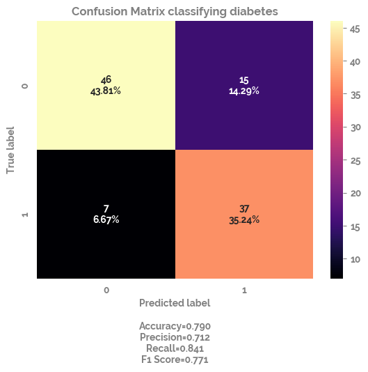
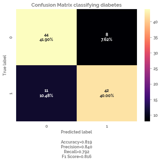
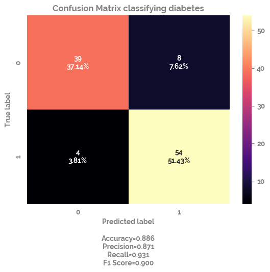
_ = make_confusion_matrix(cf=cf_matrix,
title="Confusion Matrix classifying diabetes",
sum_stats=True,
cmap="magma")
_ = plt.show()
>Train: 0=201, 1=219, Test: 0=61, 1=44
>Train: 0=210, 1=210, Test: 0=52, 1=53
>Train: 0=215, 1=205, Test: 0=47, 1=58
>Train: 0=206, 1=214, Test: 0=56, 1=49
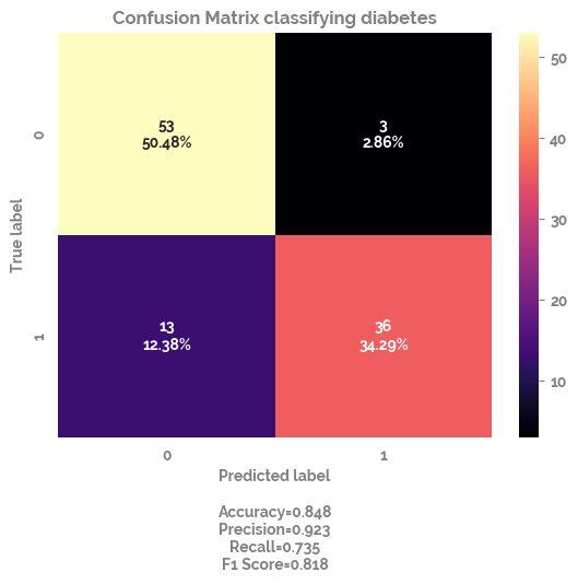
>Train: 0=216, 1=204, Test: 0=46, 1=59
[25]:
cv = RepeatedStratifiedKFold(n_splits=10, n_repeats=10, random_state=1)
[26]:
# import sklearn
# sorted(sklearn.metrics.SCORERS.keys())
[27]:
scoring_list = ('accuracy',
 'balanced_accuracy',
 'f1',
 'f1_weighted',
 'precision',
 'precision_weighted',
 'recall',
 'recall_weighted',
 'roc_auc',
               )
[28]:
tmp_out = cross_validate(optimized_rf,
                         X,
                         y,
                         scoring=scoring_list,
                         return_train_score=False,
                         cv=cv,
                         n_jobs=-1,
#                         fit_params={"sample_weight": sampling_weights} # fit_params is returning nans for some reason :/
                        )
[29]:
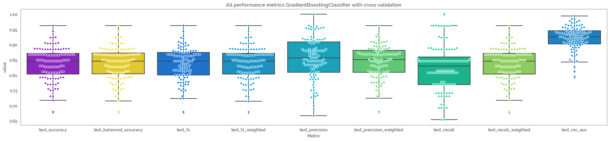
pd.DataFrame(tmp_out).drop(["fit_time", "score_time"], axis=1).agg(["mean", "median", "std"]).round(3)
[29]:
| test_accuracy | test_balanced_accuracy | test_f1 | test_f1_weighted | test_precision | test_precision_weighted | test_recall | test_recall_weighted | test_roc_auc | |
|---|---|---|---|---|---|---|---|---|---|
| mean | 0.838 | 0.838 | 0.836 | 0.838 | 0.854 | 0.843 | 0.824 | 0.838 | 0.922 |
| median | 0.846 | 0.846 | 0.846 | 0.846 | 0.857 | 0.851 | 0.830 | 0.846 | 0.926 |
| std | 0.053 | 0.053 | 0.054 | 0.054 | 0.070 | 0.053 | 0.076 | 0.053 | 0.038 |
[30]:
cv_metrics_df = pd.DataFrame(tmp_out).drop(["fit_time", "score_time"], axis=1).melt(var_name="Metric")
[31]:
_ = plt.figure(figsize=(25,5))
_ = sns.boxplot(data = cv_metrics_df,
                x = "Metric",
                y = "value")
_ = sns.swarmplot(data = cv_metrics_df,
                x = "Metric",
                y = "value", edgecolor="white", linewidth=1)
_ = plt.title(f"All performance metrics {optimized_rf.__class__.__name__} with cross validation")
[32]:
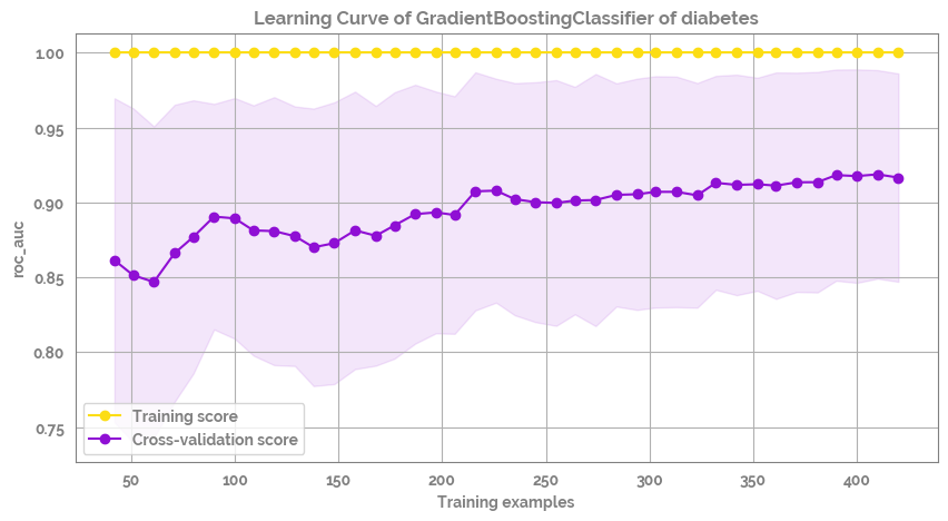
fig = plot_learning_curve(estimator=clf,
                          title=f'Learning Curve of {optimized_rf.__class__.__name__} of diabetes',
                          X=X,
                          y=y,
                          groups=None,
                          cross_color=JmsColors.PURPLE,
                          test_color=JmsColors.YELLOW,
                          scoring='roc_auc',
                          ylim=None,
                          cv=None,
                          n_jobs=10,
                          train_sizes=np.linspace(.1, 1.0, 40),
                          figsize=(10,5))
# _ = plt.savefig(f"images/learning_curve_diabetes.png", dpi=400, bbox_inches="tight")
[33]:
# X_train, X_test, y_train, y_test = train_test_split(X, y, test_size=.3, random_state=42)
# _ = optimized_rf.fit(X_train, y_train) # train the model
# y_pred = optimized_rf.predict(X_test) # predict the test data
# y_pred_proba = optimized_rf.predict_proba(X_test)[:, 1] # predict the test data

# fpr, tpr, thresholds = roc_curve(y_test, y_pred_proba, pos_label=1, drop_intermediate=True)

# auc_score = auc(fpr,tpr)

# _ = plt.figure(figsize=(7,6))
# _ = plt.plot(fpr, tpr)
# _ = plt.scatter(fpr, tpr)
# _ = plt.annotate(xy=(0.9, 0.1), s=f"AUC: {round(auc_score,3)}", ha="center")
# _ = plt.plot([0,1], [0, 1], c="grey", ls="--")
# _ = plt.title(f'ROC curve {str(optimized_rf).split("(")[0]} - diabetes classification')
# _ = sns.despine()
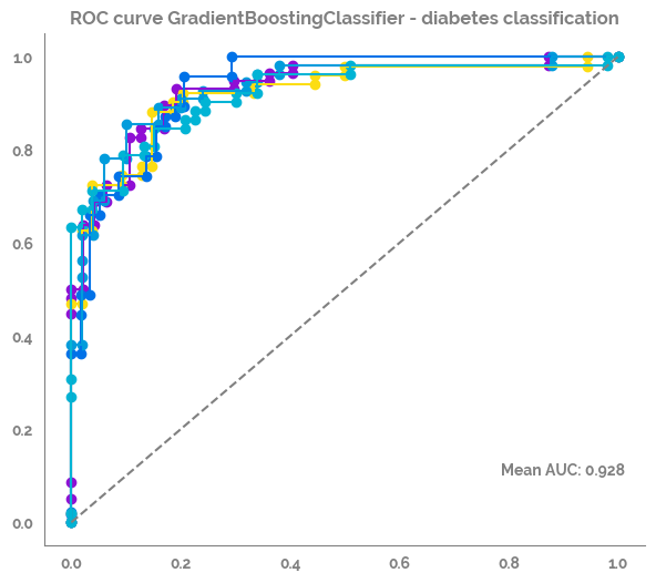
[34]:
kfold = KFold(n_splits=5, shuffle=True, random_state=42)
auc_score_list = list()
# enumerate the splits and summarize the distributions
_ = plt.figure(figsize=(7,6))
for train_ix, test_ix in kfold.split(X):
    # select rows
    X_train, X_test = X.loc[train_ix, :], X.loc[test_ix, :]
    y_train, y_test = y.loc[train_ix], y.loc[test_ix]

    _ = optimized_rf.fit(X_train, y_train) # train the model
    y_pred = optimized_rf.predict(X_test) # predict the test data
    y_pred_proba = optimized_rf.predict_proba(X_test)[:, 1] # predict the test data

    fpr, tpr, thresholds = roc_curve(y_test, y_pred_proba, pos_label=1, drop_intermediate=True)

    auc_score = auc(fpr,tpr)
    print(auc_score)

    auc_score_list.append(auc_score)

    _ = plt.plot(fpr, tpr)
    _ = plt.scatter(fpr, tpr)

_ = plt.annotate(xy=(0.9, 0.1), text=f"Mean AUC: {round(np.mean(auc_score_list),3)}", ha="center")
_ = plt.plot([0,1], [0, 1], c="grey", ls="--")
_ = plt.title(f'ROC curve {optimized_rf.__class__.__name__} - diabetes classification')
_ = sns.despine()
0.9306676449009538
0.920479302832244
0.9369038884812912
0.9309090909090908
0.9216255442670538
[35]:
X = df[feature_selected]
y = df[target]
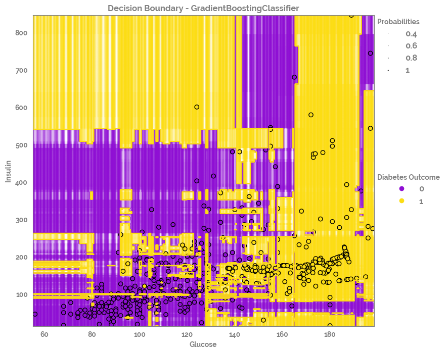
[36]:
_ = plot_decision_boundary(X=X,
                           y=y,
                           clf=optimized_rf,
                           title = f'Decision Boundary - {optimized_rf.__class__.__name__}',
                           legend_title = "Diabetes Outcome",
                          h=0.5,
                          figsize=(10, 8))