first order and second order ordinary differential equations (ODE)s
[14]:
import numpy as np
import pandas as pd
import matplotlib.pyplot as plt
import seaborn as sns
import session_info
from jmspack.utils import JmsColors
[2]:
from skmid.models import generate_model_attributes, DynamicModel
from skmid.integrator import RungeKutta4
[3]:
if "jms_style_sheet" in plt.style.available:
    plt.style.use("jms_style_sheet")
[4]:
session_info.show()
[4]:
Click to view session information
-----
matplotlib          3.5.1
numpy               1.20.3
pandas              1.4.2
seaborn             0.11.0
session_info        1.0.0
skmid               0.0.0
-----
Click to view modules imported as dependencies
PIL                 8.0.0
appnope             0.1.0
backcall            0.2.0
beta_ufunc          NA
binom_ufunc         NA
bottleneck          1.3.2
casadi              3.5.5
cffi                1.14.3
colorama            0.4.4
cycler              0.10.0
cython_runtime      NA
dateutil            2.8.1
decorator           4.4.2
ipykernel           5.3.4
ipython_genutils    0.2.0
jedi                0.18.1
kiwisolver          1.2.0
mpl_toolkits        NA
nbinom_ufunc        NA
numexpr             2.7.1
packaging           20.4
parso               0.8.0
pexpect             4.8.0
pickleshare         0.7.5
prompt_toolkit      3.0.8
ptyprocess          0.6.0
pygments            2.7.1
pyparsing           2.4.7
pytz                2020.1
scipy               1.7.1
six                 1.15.0
statsmodels         0.12.0
storemagic          NA
swig_runtime_data4  NA
tornado             6.0.4
traitlets           5.0.5
wcwidth             0.2.5
zmq                 19.0.2
-----
IPython             7.18.1
jupyter_client      6.1.7
jupyter_core        4.6.3
jupyterlab          2.2.6
notebook            6.1.4
-----
Python 3.8.5 (default, Sep  4 2020, 02:22:02) [Clang 10.0.0 ]
macOS-10.16-x86_64-i386-64bit
-----
Session information updated at 2022-04-20 12:31
Initial Parameters
[6]:
# Choose an excitation signal
np.random.seed(42)
N = 2000  # Number of samples
fs = 1  # Sampling frequency [hz]
t = np.linspace(0, (N - 1) * (1 / fs), N)
m=-0.0001
c=1
x=np.arange(N)
f=5

df_input = pd.DataFrame(
    data={
        # "u1": m*x + c,
        # "u1": 2 * np.random.random(N),
        # "u2": 2 * np.random.random(N),
        "u1": np.sin(np.pi * f * x / fs),
        # "u4": 2 * np.random.random(N),
    },
    index=t,
)

x0 = [1, -1]  # Initial Condition x0 = [0;0]; [nx = 2]

parameter_dict={"N": N,
                "fs": fs,
                "t": t,
                "x0": x0}
print("Initial Parameters")
print(parameter_dict)
display(df_input.head())
print(df_input.shape)
Initial Parameters
{'N': 2000, 'fs': 1, 't': array([0.000e+00, 1.000e+00, 2.000e+00, ..., 1.997e+03, 1.998e+03,
       1.999e+03]), 'x0': [1, -1]}
| u1 | |
|---|---|
| 0.0 | 0.000000e+00 |
| 1.0 | 6.123234e-16 |
| 2.0 | -1.224647e-15 |
| 3.0 | 5.389684e-15 |
| 4.0 | -2.449294e-15 |
(2000, 1)
[7]:
_ = plt.figure(figsize=(20, 5))
_ = sns.lineplot(data=df_input
                .reset_index()
                .melt(id_vars="index"),
                x="index",
                y="value",
                hue="variable"
                )
_ = sns.despine()

1st order ODE
Symbolics
[8]:
(x, u, param) = generate_model_attributes(state_size=1, input_size=1, parameter_size=2)

# assign specific name
x0 = [0] # initial input value
kp, tp = param[0], param[1]

param_truth = [0.1, 0.5]  # ca.DM([0.1, 0.5])

rhs = [((-1/ tp)*x) + ((kp / tp)*u)] #1st order ODE
rhs
[8]:
[MX(@1=p[1], (((p[0]/@1)*u)-(x/@1)))]
Define the Dynamic Model
[9]:
sys = DynamicModel(state=x, input=u, parameter=param, model_dynamics=rhs)
sys.print_summary()
Input Summary
-----------------
states    = ['x1']
inputs    = ['u1']
parameter = ['p1', 'p2']
output    = ['x1']

Dimension Summary
-----------------
 Number of inputs: 3
  Input 0 ("x(t)"): 1x1
  Input 1 ("u(t)"): 1x1
  Input 2 ("p"): 2x1
 Number of outputs: 1
  Output 0 ("xdot(t) = f(x(t), u(t), p)"): 1x1
Run the forward simulation and save the output as a data frame
[10]:
rk4 = RungeKutta4(model=sys, fs=fs)
rk4.simulate(initial_condition=x0[0], input=df_input, parameter=param_truth)

df_sim = rk4.output_sim_

display(df_sim.head())
print(df_sim.shape)
| x1 | |
|---|---|
| 0.0 | 0.000000e+00 |
| 1.0 | 0.000000e+00 |
| 2.0 | 4.082156e-17 |
| 3.0 | -6.803593e-17 |
| 4.0 | 3.366336e-16 |
(2001, 1)
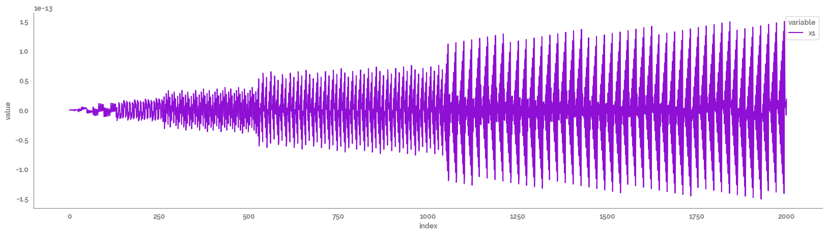
Plot the output
[11]:
_ = plt.figure(figsize=(20, 5))
_ = sns.lineplot(data=df_sim
                .reset_index()
                .melt(id_vars="index"),
                x="index",
                y="value",
                hue="variable"
                )
_ = sns.despine()
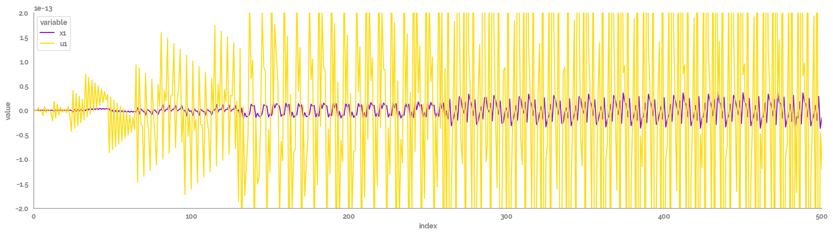
[12]:
plot_df = pd.merge(df_sim, df_input, left_index=True, right_index=True)
_ = plt.figure(figsize=(20, 5))
_ = sns.lineplot(data=plot_df
                .reset_index()
                .melt(id_vars="index"),
                x="index",
                y="value",
                hue="variable"
                )
_ = sns.despine()
_ = plt.xlim(0,500)
_ = plt.ylim(-2e-13, 2e-13)
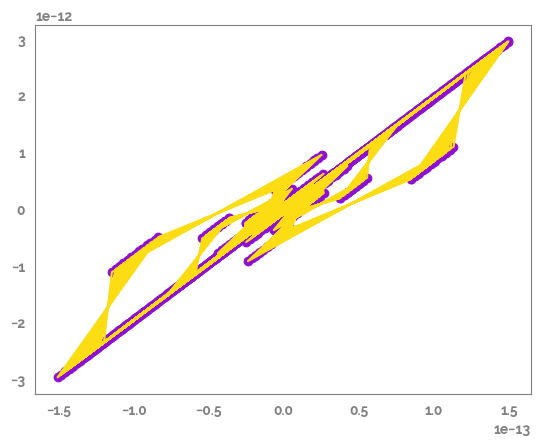
[15]:
_ = plt.scatter(df_sim.values[1:], df_input.values)
_ = plt.plot(df_sim.values[1:], df_input.values, c=JmsColors.YELLOW)
2nd order ODE
Symbolics
TODO
[ ]:
(x, u, param) = generate_model_attributes(state_size=1, input_size=1, parameter_size=2)

# assign specific name
x0 = [0] # initial input value
kp, tp = param[0], param[1]

param_truth = [0.1, 0.5]  # ca.DM([0.1, 0.5])

rhs = [((-1/ tp)*x) + ((kp / tp)*u)] #1st order ODE
rhs
Define the Dynamic Model
[ ]:
sys = DynamicModel(state=x, input=u, parameter=param, model_dynamics=rhs)
sys.print_summary()
Run the forward simulation and save the output as a data frame
[ ]:
rk4 = RungeKutta4(model=sys, fs=fs)
rk4.simulate(initial_condition=x0[0], input=df_input, parameter=param_truth)

df_sim = rk4.output_sim_

display(df_sim.head())
print(df_sim.shape)
Plot the output
[ ]:
_ = plt.figure(figsize=(20, 5))
_ = sns.lineplot(data=df_sim
                .reset_index()
                .melt(id_vars="index"),
                x="index",
                y="value",
                hue="variable"
                )
_ = sns.despine()
[ ]:
plot_df = pd.merge(df_sim, df_input, left_index=True, right_index=True)
_ = plt.figure(figsize=(20, 5))
_ = sns.lineplot(data=plot_df
                .reset_index()
                .melt(id_vars="index"),
                x="index",
                y="value",
                hue="variable"
                )
_ = sns.despine()
_ = plt.xlim(0,500)
_ = plt.ylim(-2e-13, 2e-13)
[ ]:
_ = plt.scatter(df_sim.values[1:], df_input.values)