Using a toy dataset to better understand SHapley Additive exPlanations (SHAP)
[1]:
import pandas as pd
import math
import numpy as np
import seaborn as sns
import matplotlib.pyplot as plt
import shap
from jmspack.utils import apply_scaling, JmsColors
from jmspack.ml_utils import multi_roc_auc_plot, optimize_model, plot_confusion_matrix, summary_performance_metrics_classification, plot_learning_curve, plot_decision_boundary
shap.initjs()
/opt/miniconda3/envs/ds_env/lib/python3.10/site-packages/tqdm/auto.py:22: TqdmWarning: IProgress not found. Please update jupyter and ipywidgets. See https://ipywidgets.readthedocs.io/en/stable/user_install.html
  from .autonotebook import tqdm as notebook_tqdm

[2]:
from sklearn.ensemble import RandomForestClassifier
from sklearn.linear_model import LogisticRegression
from sklearn.model_selection import cross_validate, RepeatedStratifiedKFold
[3]:
if "jms_style_sheet" in plt.style.available:
    plt.style.use("jms_style_sheet")
[4]:
df = pd.read_csv("https://raw.githubusercontent.com/mwaskom/seaborn-data/master/penguins.csv").dropna()
[5]:
df.head()
[5]:
| species | island | bill_length_mm | bill_depth_mm | flipper_length_mm | body_mass_g | sex | |
|---|---|---|---|---|---|---|---|
| 0 | Adelie | Torgersen | 39.1 | 18.7 | 181.0 | 3750.0 | MALE |
| 1 | Adelie | Torgersen | 39.5 | 17.4 | 186.0 | 3800.0 | FEMALE |
| 2 | Adelie | Torgersen | 40.3 | 18.0 | 195.0 | 3250.0 | FEMALE |
| 4 | Adelie | Torgersen | 36.7 | 19.3 | 193.0 | 3450.0 | FEMALE |
| 5 | Adelie | Torgersen | 39.3 | 20.6 | 190.0 | 3650.0 | MALE |
[6]:
df.info()
<class 'pandas.core.frame.DataFrame'>
Int64Index: 333 entries, 0 to 343
Data columns (total 7 columns):
 #   Column             Non-Null Count  Dtype
---  ------             --------------  -----
 0   species            333 non-null    object
 1   island             333 non-null    object
 2   bill_length_mm     333 non-null    float64
 3   bill_depth_mm      333 non-null    float64
 4   flipper_length_mm  333 non-null    float64
 5   body_mass_g        333 non-null    float64
 6   sex                333 non-null    object
dtypes: float64(4), object(3)
memory usage: 20.8+ KB
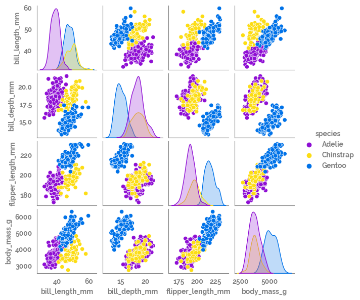
[7]:
_ = sns.pairplot(data=df, hue="species", height=1.5)
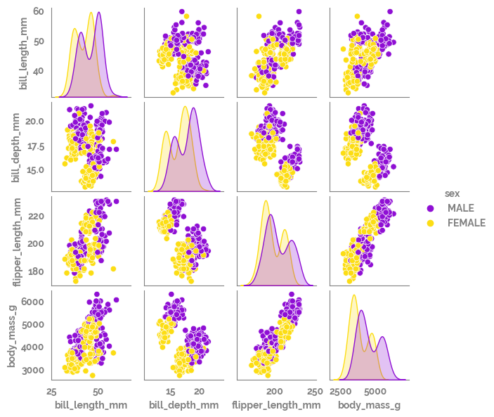
[8]:
_ = sns.pairplot(data=df, hue="sex", height=1.5)
[9]:
features_list = df.select_dtypes("number").columns.tolist()
target = "sex"
X = df[features_list]
y = df[target]
[10]:
(optimized_estimator,
feature_ranking,
feature_selected,
feature_importance,
optimized_params_df,
) = optimize_model(X=X, y=y, estimator= RandomForestClassifier(),
    grid_params_dict = {
        "max_depth": [1, 2, 3, 4, 5, 10],
        "n_estimators": [10, 20, 30, 40, 50],
        "max_features": ["log2", "auto", "sqrt"],
        "criterion": ["gini", "entropy"],
    },
    gridsearch_kwargs = {"scoring": "roc_auc", "cv": 3, "n_jobs": -2},
    rfe_kwargs = {"n_features_to_select": 2, "verbose": 1})
Fitting estimator with 4 features.
Fitting estimator with 3 features.

- Sizes :
- X shape = (333, 4)
- y shape = (333,)
- X_train shape = (233, 4)
- X_test shape = (100, 4)
- y_train shape = (233,)
- y_test shape = (100,)

- Model info :
- Optimal Parameters = {'bootstrap': True, 'ccp_alpha': 0.0, 'class_weight': None, 'criterion': 'entropy', 'max_depth': 10, 'max_features': 'auto', 'max_leaf_nodes': None, 'max_samples': None, 'min_impurity_decrease': 0.0, 'min_samples_leaf': 1, 'min_samples_split': 2, 'min_weight_fraction_leaf': 0.0, 'n_estimators': 30, 'n_jobs': None, 'oob_score': False, 'random_state': None, 'verbose': 0, 'warm_start': False}
- Selected feature list = ['bill_depth_mm', 'body_mass_g']
- Accuracy score on test set = 84.0%
[11]:
optimized_params_df
[11]:
| bootstrap | ccp_alpha | class_weight | criterion | max_depth | max_features | max_leaf_nodes | max_samples | min_impurity_decrease | min_samples_leaf | min_samples_split | min_weight_fraction_leaf | n_estimators | n_jobs | oob_score | random_state | verbose | warm_start | |
|---|---|---|---|---|---|---|---|---|---|---|---|---|---|---|---|---|---|---|
| optimal_parameters | True | 0.0 | None | entropy | 10 | auto | None | None | 0.0 | 1 | 2 | 0.0 | 30 | None | False | None | 0 | False |
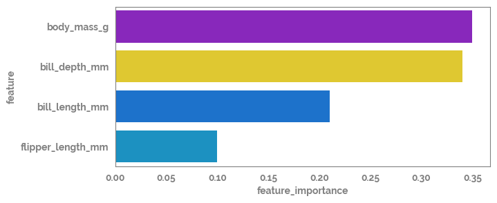
[12]:
feature_importance_df = pd.DataFrame(feature_importance.sort_values(ascending=False)).reset_index().rename(columns={"index": "feature", 0: "feature_importance"})
[13]:
_ = plt.figure(figsize=(7, 3))
_ = sns.barplot(data=feature_importance_df, x="feature_importance", y="feature")
[14]:
explainer = shap.TreeExplainer(optimized_estimator)
shap_values = explainer(X)
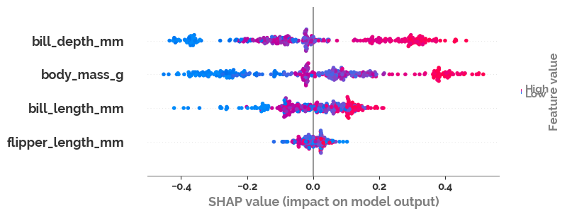
[15]:
shap.plots.beeswarm(shap_values[:, :, 1])
[16]:
shap_actual_df = pd.concat([pd.DataFrame(shap_values[:, :, 1].values, columns=features_list).melt(value_name="shap_data"),
pd.DataFrame(shap_values[:, :, 1].data, columns=features_list).melt(value_name="actual_data").drop("variable", axis=1)], axis=1)
[17]:
shap_actual_df.info()
<class 'pandas.core.frame.DataFrame'>
RangeIndex: 1332 entries, 0 to 1331
Data columns (total 3 columns):
 #   Column       Non-Null Count  Dtype
---  ------       --------------  -----
 0   variable     1332 non-null   object
 1   shap_data    1332 non-null   float64
 2   actual_data  1332 non-null   float64
dtypes: float64(2), object(1)
memory usage: 31.3+ KB
[18]:
shap_actual_df
[18]:
| variable | shap_data | actual_data | |
|---|---|---|---|
| 0 | bill_length_mm | 0.086101 | 39.1 |
| 1 | bill_length_mm | -0.023608 | 39.5 |
| 2 | bill_length_mm | 0.032321 | 40.3 |
| 3 | bill_length_mm | -0.280766 | 36.7 |
| 4 | bill_length_mm | 0.021243 | 39.3 |
| ... | ... | ... | ... |
| 1327 | body_mass_g | -0.003304 | 4925.0 |
| 1328 | body_mass_g | -0.032694 | 4850.0 |
| 1329 | body_mass_g | 0.376044 | 5750.0 |
| 1330 | body_mass_g | 0.257553 | 5200.0 |
| 1331 | body_mass_g | 0.408728 | 5400.0 |
1332 rows × 3 columns
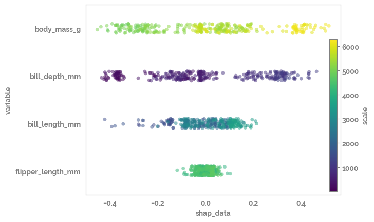
[19]:
import matplotlib
from mpl_toolkits.axes_grid1.inset_locator import inset_axes
ax = sns.stripplot(data=shap_actual_df,
                  x="shap_data",
                  y="variable",
                  hue="actual_data",
                  order=shap_actual_df.groupby("variable").var()["shap_data"].sort_values(ascending=False).index.tolist(),
                  alpha=0.5,
                  palette="viridis")
_ = plt.legend([],[], frameon=False)

N = 2
cmap = matplotlib.cm.get_cmap('viridis')
cmap_values = np.linspace(0., 1., N)
colors = cmap(cmap_values)
norm = matplotlib.colors.Normalize(vmin=shap_actual_df["actual_data"].min(), vmax=shap_actual_df["actual_data"].max())

# vertical colorbar
cbaxes = inset_axes(plt.gca(), width="3%", height="80%", loc="lower right")
cbar = matplotlib.colorbar.ColorbarBase(cbaxes, cmap=cmap,
                                        norm=norm,
                                        # ticks=ticks
                                        )
cbar.set_label('scale')
# cbar.ax.set_yticklabels(ticks, fontsize=12)
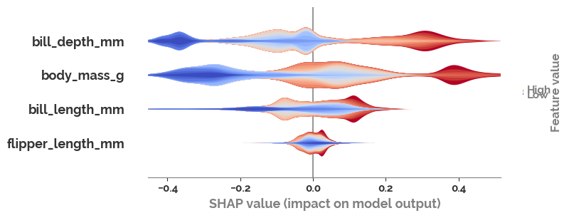
[20]:
shap.summary_plot(shap_values[:, :, 1], X, plot_type="layered_violin", color='coolwarm')
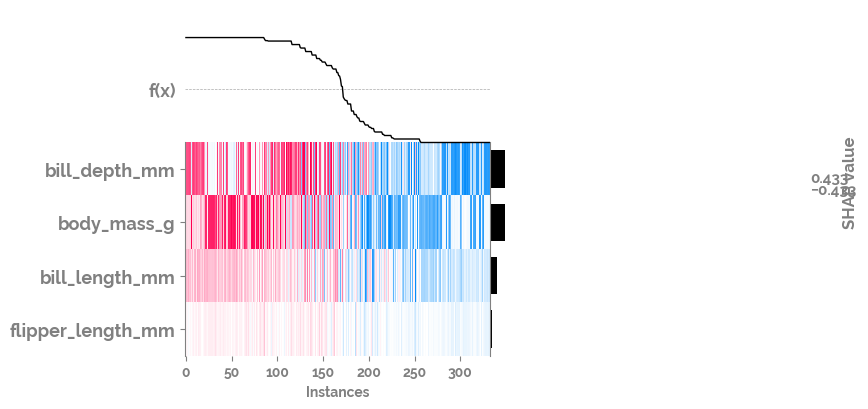
[21]:
shap.plots.heatmap(shap_values[:, :, 1], instance_order=shap_values[:, :, 1].sum(1))
[22]:
# shap.dependence_plot('bill_length_mm', shap_values.values[:, :, 0], X)
shap.force_plot(explainer.expected_value[0],
                shap_values.values[:, :, 0]
               )
[22]:
Visualization omitted, Javascript library not loaded!
Have you run `initjs()` in this notebook? If this notebook was from another user you must also trust this notebook (File -> Trust notebook). If you are viewing this notebook on github the Javascript has been stripped for security. If you are using JupyterLab this error is because a JupyterLab extension has not yet been written.
Have you run `initjs()` in this notebook? If this notebook was from another user you must also trust this notebook (File -> Trust notebook). If you are viewing this notebook on github the Javascript has been stripped for security. If you are using JupyterLab this error is because a JupyterLab extension has not yet been written.
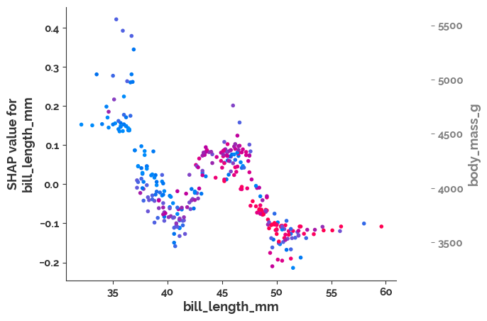
[23]:
shap.dependence_plot('bill_length_mm', shap_values.values[:, :, 0], X)
[24]:
# shap.plots.scatter(shap_values.values["bill_length_mm"], color=shap_values.values[:, :, 1])
# shap.plots.scatter(shap_values[:,"Age"])
[25]:
shap_values.values[:, :, 0]
[25]:
array([[-0.08610135, -0.27917051, -0.05639864, -0.07031806],
       [ 0.02360813,  0.22710734,  0.08169787,  0.07559811],
       [-0.03232096,  0.10554203,  0.01090091,  0.39055613],
       ...,
       [-0.10664765,  0.02194532, -0.0312427 , -0.37604353],
       [ 0.05380299,  0.33913148,  0.00596348, -0.25755317],
       [-0.11747246,  0.02249328,  0.0117189 , -0.40872828]])
[26]:
shap_values[:, :, 1]
[26]:
.values =
array([[ 0.08610135,  0.27917051,  0.05639864,  0.07031806],
       [-0.02360813, -0.22710734, -0.08169787, -0.07559811],
       [ 0.03232096, -0.10554203, -0.01090091, -0.39055613],
       ...,
       [ 0.10664765, -0.02194532,  0.0312427 ,  0.37604353],
       [-0.05380299, -0.33913148, -0.00596348,  0.25755317],
       [ 0.11747246, -0.02249328, -0.0117189 ,  0.40872828]])

.base_values =
array([0.50801144, 0.50801144, 0.50801144, 0.50801144, 0.50801144,
       0.50801144, 0.50801144, 0.50801144, 0.50801144, 0.50801144,
       0.50801144, 0.50801144, 0.50801144, 0.50801144, 0.50801144,
       0.50801144, 0.50801144, 0.50801144, 0.50801144, 0.50801144,
       0.50801144, 0.50801144, 0.50801144, 0.50801144, 0.50801144,
       0.50801144, 0.50801144, 0.50801144, 0.50801144, 0.50801144,
       0.50801144, 0.50801144, 0.50801144, 0.50801144, 0.50801144,
       0.50801144, 0.50801144, 0.50801144, 0.50801144, 0.50801144,
       0.50801144, 0.50801144, 0.50801144, 0.50801144, 0.50801144,
       0.50801144, 0.50801144, 0.50801144, 0.50801144, 0.50801144,
       0.50801144, 0.50801144, 0.50801144, 0.50801144, 0.50801144,
       0.50801144, 0.50801144, 0.50801144, 0.50801144, 0.50801144,
       0.50801144, 0.50801144, 0.50801144, 0.50801144, 0.50801144,
       0.50801144, 0.50801144, 0.50801144, 0.50801144, 0.50801144,
       0.50801144, 0.50801144, 0.50801144, 0.50801144, 0.50801144,
       0.50801144, 0.50801144, 0.50801144, 0.50801144, 0.50801144,
       0.50801144, 0.50801144, 0.50801144, 0.50801144, 0.50801144,
       0.50801144, 0.50801144, 0.50801144, 0.50801144, 0.50801144,
       0.50801144, 0.50801144, 0.50801144, 0.50801144, 0.50801144,
       0.50801144, 0.50801144, 0.50801144, 0.50801144, 0.50801144,
       0.50801144, 0.50801144, 0.50801144, 0.50801144, 0.50801144,
       0.50801144, 0.50801144, 0.50801144, 0.50801144, 0.50801144,
       0.50801144, 0.50801144, 0.50801144, 0.50801144, 0.50801144,
       0.50801144, 0.50801144, 0.50801144, 0.50801144, 0.50801144,
       0.50801144, 0.50801144, 0.50801144, 0.50801144, 0.50801144,
       0.50801144, 0.50801144, 0.50801144, 0.50801144, 0.50801144,
       0.50801144, 0.50801144, 0.50801144, 0.50801144, 0.50801144,
       0.50801144, 0.50801144, 0.50801144, 0.50801144, 0.50801144,
       0.50801144, 0.50801144, 0.50801144, 0.50801144, 0.50801144,
       0.50801144, 0.50801144, 0.50801144, 0.50801144, 0.50801144,
       0.50801144, 0.50801144, 0.50801144, 0.50801144, 0.50801144,
       0.50801144, 0.50801144, 0.50801144, 0.50801144, 0.50801144,
       0.50801144, 0.50801144, 0.50801144, 0.50801144, 0.50801144,
       0.50801144, 0.50801144, 0.50801144, 0.50801144, 0.50801144,
       0.50801144, 0.50801144, 0.50801144, 0.50801144, 0.50801144,
       0.50801144, 0.50801144, 0.50801144, 0.50801144, 0.50801144,
       0.50801144, 0.50801144, 0.50801144, 0.50801144, 0.50801144,
       0.50801144, 0.50801144, 0.50801144, 0.50801144, 0.50801144,
       0.50801144, 0.50801144, 0.50801144, 0.50801144, 0.50801144,
       0.50801144, 0.50801144, 0.50801144, 0.50801144, 0.50801144,
       0.50801144, 0.50801144, 0.50801144, 0.50801144, 0.50801144,
       0.50801144, 0.50801144, 0.50801144, 0.50801144, 0.50801144,
       0.50801144, 0.50801144, 0.50801144, 0.50801144, 0.50801144,
       0.50801144, 0.50801144, 0.50801144, 0.50801144, 0.50801144,
       0.50801144, 0.50801144, 0.50801144, 0.50801144, 0.50801144,
       0.50801144, 0.50801144, 0.50801144, 0.50801144, 0.50801144,
       0.50801144, 0.50801144, 0.50801144, 0.50801144, 0.50801144,
       0.50801144, 0.50801144, 0.50801144, 0.50801144, 0.50801144,
       0.50801144, 0.50801144, 0.50801144, 0.50801144, 0.50801144,
       0.50801144, 0.50801144, 0.50801144, 0.50801144, 0.50801144,
       0.50801144, 0.50801144, 0.50801144, 0.50801144, 0.50801144,
       0.50801144, 0.50801144, 0.50801144, 0.50801144, 0.50801144,
       0.50801144, 0.50801144, 0.50801144, 0.50801144, 0.50801144,
       0.50801144, 0.50801144, 0.50801144, 0.50801144, 0.50801144,
       0.50801144, 0.50801144, 0.50801144, 0.50801144, 0.50801144,
       0.50801144, 0.50801144, 0.50801144, 0.50801144, 0.50801144,
       0.50801144, 0.50801144, 0.50801144, 0.50801144, 0.50801144,
       0.50801144, 0.50801144, 0.50801144, 0.50801144, 0.50801144,
       0.50801144, 0.50801144, 0.50801144, 0.50801144, 0.50801144,
       0.50801144, 0.50801144, 0.50801144, 0.50801144, 0.50801144,
       0.50801144, 0.50801144, 0.50801144, 0.50801144, 0.50801144,
       0.50801144, 0.50801144, 0.50801144, 0.50801144, 0.50801144,
       0.50801144, 0.50801144, 0.50801144, 0.50801144, 0.50801144,
       0.50801144, 0.50801144, 0.50801144, 0.50801144, 0.50801144,
       0.50801144, 0.50801144, 0.50801144, 0.50801144, 0.50801144,
       0.50801144, 0.50801144, 0.50801144, 0.50801144, 0.50801144,
       0.50801144, 0.50801144, 0.50801144])

.data =
array([[  39.1,   18.7,  181. , 3750. ],
       [  39.5,   17.4,  186. , 3800. ],
       [  40.3,   18. ,  195. , 3250. ],
       ...,
       [  50.4,   15.7,  222. , 5750. ],
       [  45.2,   14.8,  212. , 5200. ],
       [  49.9,   16.1,  213. , 5400. ]])
[27]:
cv = RepeatedStratifiedKFold(n_splits=10, n_repeats=10, random_state=1)
scoring_list = ('accuracy',
 'balanced_accuracy',
 'f1',
 'f1_weighted',
 'precision',
 'precision_weighted',
 'recall',
 'recall_weighted',
 'roc_auc',
               )
[28]:
tmp_out = cross_validate(estimator=optimized_estimator, X=X[feature_selected], y=y.astype("category").cat.codes, groups=None, scoring=scoring_list, cv=cv, n_jobs=-1)
[29]:
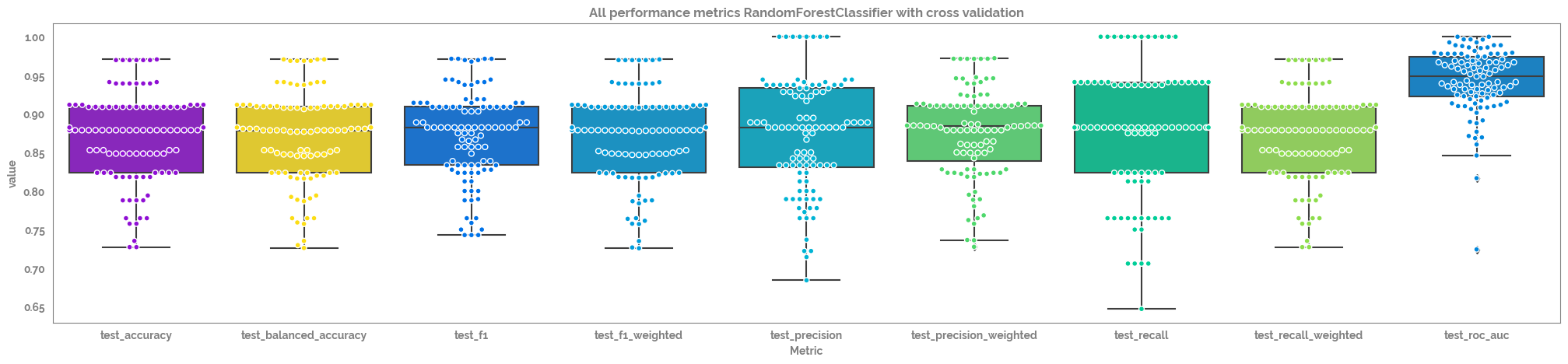
pd.DataFrame(tmp_out).drop(["fit_time", "score_time"], axis=1).agg(["mean", "median", "std"]).round(3)
[29]:
| test_accuracy | test_balanced_accuracy | test_f1 | test_f1_weighted | test_precision | test_precision_weighted | test_recall | test_recall_weighted | test_roc_auc | |
|---|---|---|---|---|---|---|---|---|---|
| mean | 0.871 | 0.871 | 0.872 | 0.870 | 0.872 | 0.876 | 0.878 | 0.871 | 0.942 |
| median | 0.879 | 0.879 | 0.882 | 0.879 | 0.882 | 0.884 | 0.882 | 0.879 | 0.949 |
| std | 0.058 | 0.058 | 0.058 | 0.058 | 0.072 | 0.057 | 0.080 | 0.058 | 0.043 |
[30]:
cv_metrics_df = pd.DataFrame(tmp_out).drop(["fit_time", "score_time"], axis=1).melt(var_name="Metric")
[31]:
_ = plt.figure(figsize=(25,5))
_ = sns.boxplot(data = cv_metrics_df,
                x = "Metric",
                y = "value")
_ = sns.swarmplot(data = cv_metrics_df,
                x = "Metric",
                y = "value", edgecolor="white", linewidth=1)
_ = plt.title(f"All performance metrics {optimized_estimator.__class__.__name__} with cross validation")
7.0% of the points cannot be placed; you may want to decrease the size of the markers or use stripplot.
15.0% of the points cannot be placed; you may want to decrease the size of the markers or use stripplot.
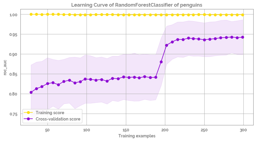
[32]:
fig = plot_learning_curve(estimator=optimized_estimator,
                          title=f'Learning Curve of {optimized_estimator.__class__.__name__} of penguins',
                          X=X[feature_selected],
                          y=y,
                          groups=None,
                          cross_color=JmsColors.PURPLE,
                          test_color=JmsColors.YELLOW,
                          scoring='roc_auc',
                          ylim=None,
                          cv=cv,
                          n_jobs=10,
                          train_sizes=np.linspace(.1, 1.0, 40),
                          figsize=(10,5))
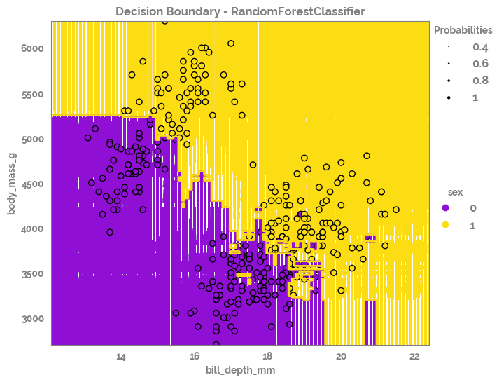
[33]:
_ = plot_decision_boundary(X=X[feature_selected],
                           y=y,
                           clf=optimized_estimator,
                           title = f'Decision Boundary - {optimized_estimator.__class__.__name__}',
                           legend_title = target,
                          h=0.1,
                          figsize=(8, 6))
[ ]: