Neural Transfer Using PyTorch
Introduction
This notebook is based on the following tutorial: https://pytorch.org/tutorials/advanced/neural_style_tutorial.html
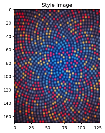
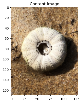
Neural-Style, or Neural-Transfer, allows you to take an image and reproduce it with a new artistic style. The algorithm takes three images, an input image, a content-image, and a style-image, and changes the input to resemble the content of the content-image and the artistic style of the style-image.
Underlying Principle
The principle is simple: we define two distances, one for the content (\(D_C\)) and one for the style (\(D_S\)). \(D_C\) measures how different the content is between two images while \(D_S\) measures how different the style is between two images. Then, we take a third image, the input, and transform it to minimize both its content-distance with the content-image and its style-distance with the style-image. Now we can import the necessary packages and begin the neural transfer.
Importing Packages and Selecting a Device
Below is a list of the packages needed to implement the neural transfer.
torch,torch.nn,numpy(indispensables packages for neural networks with PyTorch)torch.optim(efficient gradient descents)PIL,PIL.Image,matplotlib.pyplot(load and display images)torchvision.transforms(transform PIL images into tensors)torchvision.models(train or load pre-trained models)copy(to deep copy the models; system package)see the
requirements.txtfile in this folder
[1]:
from __future__ import print_function

import torch
import torch.nn as nn
import torch.nn.functional as F
import torch.optim as optim

from PIL import Image
import matplotlib.pyplot as plt

import torchvision.transforms as transforms
import torchvision.models as models
import torchvision.transforms.functional as fn

import copy
Next, we need to choose which device to run the network on and import the content and style images. Running the neural transfer algorithm on large images takes longer and will go much faster when running on a GPU. We can use torch.cuda.is_available() to detect if there is a GPU available. Next, we set the torch.device for use throughout the tutorial. Also the .to(device) method is used to move tensors or modules to a desired device.
[2]:
device = torch.device("cuda" if torch.cuda.is_available() else "cpu")
device
[2]:
device(type='cpu')
Loading the Images
Now we will import the style and content images. The original PIL images have values between 0 and 255, but when transformed into torch tensors, their values are converted to be between 0 and 1. The images also need to be resized to have the same dimensions. An important detail to note is that neural networks from the torch library are trained with tensor values ranging from 0 to 1. If you try to feed the networks with 0 to 255 tensor images, then the activated feature maps will be unable to sense the intended content and style. However, pre-trained networks from the Caffe library are trained with 0 to 255 tensor images.
[3]:
# desired size of the output image
imsize = 512 if torch.cuda.is_available() else 128  # use small size if no gpu

loader = transforms.Compose([
    transforms.Resize(imsize),  # scale imported image
    transforms.ToTensor()])  # transform it into a torch tensor


def image_loader(image_name):
    image = Image.open(image_name)
    # fake batch dimension required to fit network's input dimensions
    image = loader(image).unsqueeze(0)
    return image.to(device, torch.float)


style_img = image_loader("images/style_img.jpg")
content_img = image_loader("images/content_img.jpg")

try:
    assert style_img.size() == content_img.size()
except:
    print("we need to import style and content images of the same size")
    print(f"Style Image size: {style_img.size()}")
    print(f"Content Image size: {content_img.size()}")
we need to import style and content images of the same size
Style Image size: torch.Size([1, 3, 157, 128])
Content Image size: torch.Size([1, 3, 170, 128])
[4]:
style_img = fn.resize(style_img, size=[170, 128])
style_img.size()
[4]:
torch.Size([1, 3, 170, 128])
[5]:
content_img.size()
[5]:
torch.Size([1, 3, 170, 128])
[6]:
assert style_img.size() == content_img.size(), \
    "we need to import style and content images of the same size"
Now, let’s create a function that displays an image by reconverting a copy of it to PIL format and displaying the copy using plt.imshow. We will try displaying the content and style images to ensure they were imported correctly.
[7]:
unloader = transforms.ToPILImage()  # reconvert into PIL image

plt.ion()

def imshow(tensor, title=None):
    image = tensor.cpu().clone()  # we clone the tensor to not do changes on it
    image = image.squeeze(0)      # remove the fake batch dimension
    image = unloader(image)
    fig, ax = plt.subplots()
    plt.imshow(image)
    if title is not None:
        plt.title(title)
    plt.pause(0.001) # pause a bit so that plots are updated

    return image


# plt.figure()
_ = imshow(style_img, title='Style Image')

# plt.figure()
_ = imshow(content_img, title='Content Image')
Loss Functions
Content Loss ~~~~~~~~~~~~
The content loss is a function that represents a weighted version of the content distance for an individual layer. The function takes the feature maps \(F_{XL}\) of a layer \(L\) in a network processing input \(X\) and returns the weighted content distance \(w_{CL}.D_C^L(X,C)\) between the image \(X\) and the content image \(C\). The feature maps of the content image(\(F_{CL}\)) must be known by the function in order to calculate the content distance. We implement
this function as a torch module with a constructor that takes \(F_{CL}\) as an input. The distance \(\|F_{XL} - F_{CL}\|^2\) is the mean square error between the two sets of feature maps, and can be computed using nn.MSELoss.
We will add this content loss module directly after the convolution layer(s) that are being used to compute the content distance. This way each time the network is fed an input image the content losses will be computed at the desired layers and because of auto grad, all the gradients will be computed. Now, in order to make the content loss layer transparent we must define a forward method that computes the content loss and then returns the layer’s input. The computed loss is saved as a
parameter of the module.
[8]:
class ContentLoss(nn.Module):

    def __init__(self, target,):
        super(ContentLoss, self).__init__()
        # we 'detach' the target content from the tree used
        # to dynamically compute the gradient: this is a stated value,
        # not a variable. Otherwise the forward method of the criterion
        # will throw an error.
        self.target = target.detach()

    def forward(self, input):
        self.loss = F.mse_loss(input, self.target)
        return input
Style Loss ~~~~~~~~~~
The style loss module is implemented similarly to the content loss module. It will act as a transparent layer in a network that computes the style loss of that layer. In order to calculate the style loss, we need to compute the gram matrix \(G_{XL}\). A gram matrix is the result of multiplying a given matrix by its transposed matrix. In this application the given matrix is a reshaped version of the feature maps \(F_{XL}\) of a layer \(L\). \(F_{XL}\) is reshaped to form \(\hat{F}_{XL}\), a \(K\) x \(N\) matrix, where \(K\) is the number of feature maps at layer \(L\) and \(N\) is the length of any vectorized feature map \(F_{XL}^k\). For example, the first line of \(\hat{F}_{XL}\) corresponds to the first vectorized feature map \(F_{XL}^1\).
Finally, the gram matrix must be normalized by dividing each element by the total number of elements in the matrix. This normalization is to counteract the fact that \(\hat{F}_{XL}\) matrices with a large \(N\) dimension yield larger values in the Gram matrix. These larger values will cause the first layers (before pooling layers) to have a larger impact during the gradient descent. Style features tend to be in the deeper layers of the network so this normalization step is crucial.
[9]:
def gram_matrix(input):
    a, b, c, d = input.size()  # a=batch size(=1)
    # b=number of feature maps
    # (c,d)=dimensions of a f. map (N=c*d)

    features = input.view(a * b, c * d)  # resise F_XL into \hat F_XL

    G = torch.mm(features, features.t())  # compute the gram product

    # we 'normalize' the values of the gram matrix
    # by dividing by the number of element in each feature maps.
    return G.div(a * b * c * d)
Now the style loss module looks almost exactly like the content loss module. The style distance is also computed using the mean square error between \(G_{XL}\) and \(G_{SL}\).
[10]:
class StyleLoss(nn.Module):

    def __init__(self, target_feature):
        super(StyleLoss, self).__init__()
        self.target = gram_matrix(target_feature).detach()

    def forward(self, input):
        G = gram_matrix(input)
        self.loss = F.mse_loss(G, self.target)
        return input
Importing the Model
Now we need to import a pre-trained neural network. We will use a 19 layer VGG network like the one used in the paper.
PyTorch’s implementation of VGG is a module divided into two child Sequential modules: features (containing convolution and pooling layers), and classifier (containing fully connected layers). We will use the features module because we need the output of the individual convolution layers to measure content and style loss. Some layers have different behavior during training than evaluation, so we must set the network to evaluation mode using .eval().
[11]:
cnn = models.vgg19(pretrained=True).features.to(device).eval()
/Users/james/miniconda3/envs/ds_env/lib/python3.9/site-packages/torchvision/models/_utils.py:208: UserWarning: The parameter 'pretrained' is deprecated since 0.13 and will be removed in 0.15, please use 'weights' instead.
  warnings.warn(
/Users/james/miniconda3/envs/ds_env/lib/python3.9/site-packages/torchvision/models/_utils.py:223: UserWarning: Arguments other than a weight enum or `None` for 'weights' are deprecated since 0.13 and will be removed in 0.15. The current behavior is equivalent to passing `weights=VGG19_Weights.IMAGENET1K_V1`. You can also use `weights=VGG19_Weights.DEFAULT` to get the most up-to-date weights.
  warnings.warn(msg)
Additionally, VGG networks are trained on images with each channel normalized by mean=[0.485, 0.456, 0.406] and std=[0.229, 0.224, 0.225]. We will use them to normalize the image before sending it into the network.
[12]:
cnn_normalization_mean = torch.tensor([0.485, 0.456, 0.406]).to(device)
cnn_normalization_std = torch.tensor([0.229, 0.224, 0.225]).to(device)

# create a module to normalize input image so we can easily put it in a
# nn.Sequential
class Normalization(nn.Module):
    def __init__(self, mean, std):
        super(Normalization, self).__init__()
        # .view the mean and std to make them [C x 1 x 1] so that they can
        # directly work with image Tensor of shape [B x C x H x W].
        # B is batch size. C is number of channels. H is height and W is width.
        self.mean = torch.tensor(mean).view(-1, 1, 1)
        self.std = torch.tensor(std).view(-1, 1, 1)

    def forward(self, img):
        # normalize img
        return (img - self.mean) / self.std
A Sequential module contains an ordered list of child modules. For instance, vgg19.features contains a sequence (Conv2d, ReLU, MaxPool2d, Conv2d, ReLU…) aligned in the right order of depth. We need to add our content loss and style loss layers immediately after the convolution layer they are detecting. To do this we must create a new Sequential module that has content loss and style loss modules correctly inserted.
[13]:
# desired depth layers to compute style/content losses :
content_layers_default = ['conv_4']
style_layers_default = ['conv_1', 'conv_2',
                        'conv_3', 'conv_4',
                        'conv_5', 'conv_6',
                        'conv_7', 'conv_8',
                        'conv_9', 'conv_10']

def get_style_model_and_losses(cnn,
                                normalization_mean,
                                normalization_std,
                               style_img,
                               content_img,
                               content_layers=content_layers_default,
                               style_layers=style_layers_default):
    # normalization module
    normalization = Normalization(normalization_mean, normalization_std).to(device)

    # just in order to have an iterable access to or list of content/syle
    # losses
    content_losses = []
    style_losses = []

    # assuming that cnn is a nn.Sequential, so we make a new nn.Sequential
    # to put in modules that are supposed to be activated sequentially
    model = nn.Sequential(normalization)

    i = 0  # increment every time we see a conv
    for layer in cnn.children():
        if isinstance(layer, nn.Conv2d):
            i += 1
            name = 'conv_{}'.format(i)
        elif isinstance(layer, nn.ReLU):
            name = 'relu_{}'.format(i)
            # The in-place version doesn't play very nicely with the ContentLoss
            # and StyleLoss we insert below. So we replace with out-of-place
            # ones here.
            layer = nn.ReLU(inplace=False)
        elif isinstance(layer, nn.MaxPool2d):
            name = 'pool_{}'.format(i)
        elif isinstance(layer, nn.BatchNorm2d):
            name = 'bn_{}'.format(i)
        else:
            raise RuntimeError('Unrecognized layer: {}'.format(layer.__class__.__name__))

        model.add_module(name, layer)

        if name in content_layers:
            # add content loss:
            target = model(content_img).detach()
            content_loss = ContentLoss(target)
            model.add_module("content_loss_{}".format(i), content_loss)
            content_losses.append(content_loss)

        if name in style_layers:
            # add style loss:
            target_feature = model(style_img).detach()
            style_loss = StyleLoss(target_feature)
            model.add_module("style_loss_{}".format(i), style_loss)
            style_losses.append(style_loss)

    # now we trim off the layers after the last content and style losses
    for i in range(len(model) - 1, -1, -1):
        if isinstance(model[i], ContentLoss) or isinstance(model[i], StyleLoss):
            break

    model = model[:(i + 1)]

    return model, style_losses, content_losses
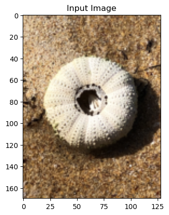
Next, we select the input image. You can use a copy of the content image or white noise.
[14]:
input_img = content_img.clone()
# if you want to use white noise instead uncomment the below line:
# input_img = torch.randn(content_img.data.size(), device=device)

# add the original input image to the figure:
_ = imshow(input_img, title='Input Image')
Gradient Descent
As Leon Gatys, the author of the algorithm, suggested here <https://discuss.pytorch.org/t/pytorch-tutorial-for-neural-transfert-of-artistic-style/336/20?u=alexis-jacq>__, we will use L-BFGS algorithm to run our gradient descent. Unlike training a network, we want to train the input image in order to minimise the content/style losses. We will create a PyTorch L-BFGS optimizer optim.LBFGS and pass our image to it as the tensor to optimize.
[15]:
def get_input_optimizer(input_img):
    # this line to show that input is a parameter that requires a gradient
    optimizer = optim.LBFGS([input_img])
    return optimizer
Finally, we must define a function that performs the neural transfer. For each iteration of the networks, it is fed an updated input and computes new losses. We will run the backward methods of each loss module to dynamicaly compute their gradients. The optimizer requires a “closure” function, which reevaluates the module and returns the loss.
We still have one final constraint to address. The network may try to optimize the input with values that exceed the 0 to 1 tensor range for the image. We can address this by correcting the input values to be between 0 to 1 each time the network is run.
[16]:
def run_style_transfer(cnn,
                        normalization_mean,
                        normalization_std,
                       content_img,
                       style_img,
                       input_img,
                       num_steps=1000,
                       style_weight=1000000, content_weight=1):
    """Run the style transfer."""
    print('Building the style transfer model..')
    model, style_losses, content_losses = get_style_model_and_losses(cnn,
        normalization_mean, normalization_std, style_img, content_img)

    # We want to optimize the input and not the model parameters so we
    # update all the requires_grad fields accordingly
    input_img.requires_grad_(True)
    model.requires_grad_(False)

    optimizer = get_input_optimizer(input_img)

    print('Optimizing..')
    run = [0]
    while run[0] <= num_steps:

        def closure():
            # correct the values of updated input image
            with torch.no_grad():
                input_img.clamp_(0, 1)

            optimizer.zero_grad()
            model(input_img)
            style_score = 0
            content_score = 0

            for sl in style_losses:
                style_score += sl.loss
            for cl in content_losses:
                content_score += cl.loss

            style_score *= style_weight
            content_score *= content_weight

            loss = style_score + content_score
            loss.backward()

            run[0] += 1
            if run[0] % 100 == 0:
                print("run {}:".format(run))
                print('Style Loss : {:4f} Content Loss: {:4f}'.format(
                    style_score.item(), content_score.item()))
                print()

            return style_score + content_score

        optimizer.step(closure)

    # a last correction...
    with torch.no_grad():
        input_img.clamp_(0, 1)

    return input_img
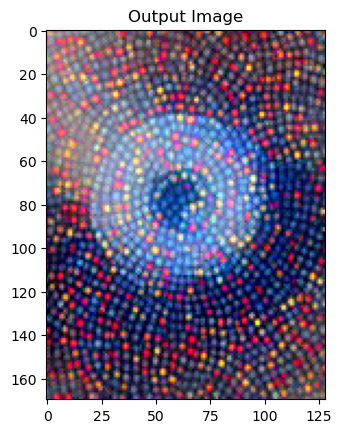
Finally, we can run the algorithm.
[20]:
output = run_style_transfer(cnn,
                            cnn_normalization_mean,
                            cnn_normalization_std,
                            content_img,
                            style_img,
                            input_img,
                            num_steps=500,
                            style_weight=1000000 #1000000
                            )

# plt.figure()
# imshow(output, title='Output Image')

# # sphinx_gallery_thumbnail_number = 4
# plt.ioff()
# plt.show()
Building the style transfer model..
/var/folders/76/w4hjx50937lb151qm8l0xq_w0000gn/T/ipykernel_73027/1744401072.py:12: UserWarning: To copy construct from a tensor, it is recommended to use sourceTensor.clone().detach() or sourceTensor.clone().detach().requires_grad_(True), rather than torch.tensor(sourceTensor).
  self.mean = torch.tensor(mean).view(-1, 1, 1)
/var/folders/76/w4hjx50937lb151qm8l0xq_w0000gn/T/ipykernel_73027/1744401072.py:13: UserWarning: To copy construct from a tensor, it is recommended to use sourceTensor.clone().detach() or sourceTensor.clone().detach().requires_grad_(True), rather than torch.tensor(sourceTensor).
  self.std = torch.tensor(std).view(-1, 1, 1)
Optimizing..
run [100]:
Style Loss : 474.479095 Content Loss: 62.232918

run [200]:
Style Loss : 378.271027 Content Loss: 65.982285

run [300]:
Style Loss : 306.477478 Content Loss: 67.984390

run [400]:
Style Loss : 258.166260 Content Loss: 69.344818

run [500]:
Style Loss : 240.144394 Content Loss: 70.163918
[21]:
mixed = imshow(output, title='Output Image')
[22]:
mixed.resize((600, 800)).save("images/mixed_img.png", quality=400)