Stress prediction based on biometrics data
Author: James Twose Date: 20-03-2021
This dataset comprises of heart rate variability (HRV) and Electrodermal activity (EDA) computed from the SWELL1 and the WESAD2 datasets. It comprises of the following three directories and sub-directories: 1) interim —contains the intermediate data that has been transformed directly from the raw datasets. The raw datasets are not included but they can be obtained from their respective publishers. This folder contains the following major contents: - a) Labels —the ground truth of the experiments. For the details of how these were obtained, please refer to the papers included in the root of this director. - b) eda —the raw eda signals - c) rri —the inter-beat (RR) interval extracted from the electrocardiogram (ECG) signal 2) processed —containes files that were computed from those in the intermidiate directory facilitate the analysis
final —files that were used for creating the model. This directory contains two sub-directories:
datasets —contains the combined train, test a nd validation data used to create the model. For more details refer to section II of the paper ”The influence of person-specific biometrics in improving generic stress predictive models”
results —contains the detailed results published in ”The influence of person-specific biometrics in improving generic stress predictive models”
Targets:
NASA-TLX for the SWELL
SSSQ for the WESAD
Import all necessary packages and functions
[66]:
# utility packages
import sys
import os
import glob
from sinfo import sinfo
# import warnings

# data manipulation packages
import pandas as pd
# from pandas.io.json import json_normalize #package for flattening json in pandas df
# from ast import literal_eval
import numpy as np

# plotting packages
import matplotlib.pyplot as plt
import matplotlib.patches as patches
import seaborn as sns

# analysis packages
from sklearn.preprocessing import MinMaxScaler
from sklearn.feature_selection import VarianceThreshold
from jmspack.NLTSA import ts_levels

# internal script
from extras import (swell_eda_features_cols,
                   swell_eda_target_cols,
                   variance_threshold,
                   nunique_threshold)
[11]:
sinfo(write_req_file=False)
-----
extras      NA
jmspack     0.0.2
matplotlib  3.3.4
numpy       1.19.2
pandas      1.2.3
seaborn     0.11.1
sinfo       0.3.1
sklearn     0.23.2
-----
IPython             7.21.0
jupyter_client      6.1.7
jupyter_core        4.7.1
jupyterlab          3.0.10
notebook            6.2.0
-----
Python 3.8.8 (default, Feb 24 2021, 13:46:16) [Clang 10.0.0 ]
macOS-10.16-x86_64-i386-64bit
12 logical CPU cores, i386
-----
Session information updated at 2021-03-21 15:35
Read in data
[142]:
# df_names_list = glob.glob("dataset/1. processed/eda/swell/*.xlsx")

# df = pd.DataFrame()
# for df_name in df_names_list:
#     current_df = pd.read_excel(df_name)
#     current_df["user_id"] = int(df_name.split("/")[-1].split(".")[0][1:])
#     df = pd.concat([df, current_df], axis=0)

# df = (df
#  .sort_values(["user_id", "Time"])
#  .loc[:, ["user_id"] + [x for x in df.drop("user_id", axis=1).columns.tolist()]]
#  .reset_index(drop=True)
# )

# df.to_csv("swell_eda_all_participants.csv")

df = pd.read_csv("swell_eda_all_participants.csv",
                index_col=0)
[170]:
df.shape
[170]:
(104053, 37)
[143]:
df.info()
<class 'pandas.core.frame.DataFrame'>
Int64Index: 104053 entries, 0 to 104052
Data columns (total 37 columns):
 #   Column          Non-Null Count   Dtype
---  ------          --------------   -----
 0   user_id         104053 non-null  int64
 1   Time            104053 non-null  float64
 2   MEAN            104053 non-null  float64
 3   MAX             104053 non-null  float64
 4   MIN             104053 non-null  float64
 5   RANGE           104053 non-null  float64
 6   KURT            104053 non-null  float64
 7   SKEW            104053 non-null  float64
 8   MEAN_1ST_GRAD   104053 non-null  float64
 9   STD_1ST_GRAD    104053 non-null  float64
 10  MEAN_2ND_GRAD   104053 non-null  float64
 11  STD_2ND_GRAD    104053 non-null  float64
 12  ALSC            104053 non-null  float64
 13  INSC            104053 non-null  float64
 14  APSC            104053 non-null  float64
 15  RMSC            104053 non-null  float64
 16  MIN_PEAKS       104053 non-null  float64
 17  MAX_PEAKS       104053 non-null  float64
 18  STD_PEAKS       104053 non-null  float64
 19  MEAN_PEAKS      104053 non-null  float64
 20  MIN_ONSET       104053 non-null  float64
 21  MAX_ONSET       104053 non-null  float64
 22  STD_ONSET       104053 non-null  float64
 23  MEAN_ONSET      104053 non-null  float64
 24  condition       104053 non-null  object
 25  Valence         104053 non-null  int64
 26  Arousal         104053 non-null  int64
 27  Dominance       104053 non-null  int64
 28  Stress          104053 non-null  float64
 29  MentalEffort    104053 non-null  float64
 30  MentalDemand    104053 non-null  float64
 31  PhysicalDemand  104053 non-null  float64
 32  TemporalDemand  104053 non-null  float64
 33  Effort          104053 non-null  float64
 34  Performance     104053 non-null  float64
 35  Frustration     104053 non-null  float64
 36  NasaTLX         98494 non-null   float64
dtypes: float64(32), int64(4), object(1)
memory usage: 30.2+ MB
Exploratory Data Analysis (EDA)
[157]:
TARGET = "NasaTLX"
[158]:
df[swell_eda_features_cols] = pd.DataFrame(MinMaxScaler()
             .fit_transform(
                 df[swell_eda_features_cols]
             ),
             columns=swell_eda_features_cols)
[159]:
target_df = (df[["user_id"]+swell_eda_target_cols]
 .groupby(["user_id", "condition"])
 .mean()
             .reset_index()
)
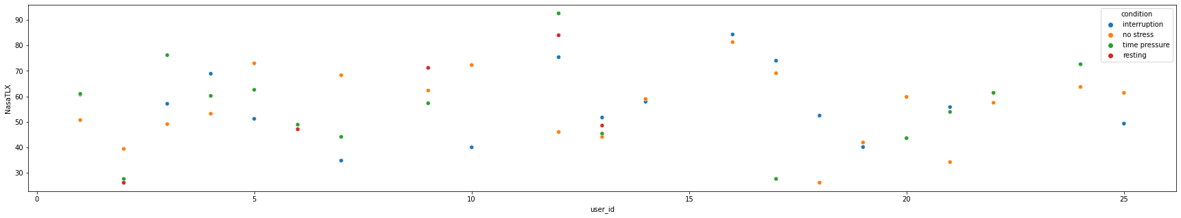
[175]:
_ = plt.figure(figsize=(30, 5))
_ = sns.scatterplot(x="user_id",
                    y=TARGET,
                    hue="condition",
                    data=target_df)
[179]:
target_df.groupby("user_id").count()[TARGET].value_counts()
[179]:
2    8
3    8
4    5
0    1
Name: NasaTLX, dtype: int64
[167]:
target_df.groupby("condition").describe()[TARGET]
[167]:
| count | mean | std | min | 25% | 50% | 75% | max | |
|---|---|---|---|---|---|---|---|---|
| condition | ||||||||
| interruption | 18.0 | 55.448197 | 15.246596 | 26.1 | 47.6500 | 54.123876 | 66.85 | 84.319786 |
| no stress | 21.0 | 55.209524 | 13.978838 | 26.1 | 46.0000 | 57.500000 | 63.70 | 81.300000 |
| resting | 6.0 | 56.391667 | 20.356827 | 26.1 | 47.4625 | 54.975000 | 68.75 | 84.000000 |
| time pressure | 15.0 | 55.666227 | 17.349646 | 27.6 | 44.7500 | 57.300000 | 62.00 | 92.600000 |
[115]:
# plot_df = (df
#  .loc[df["user_id"] == 1, ["user_id"]+swell_eda_features_cols]
#  .sample(frac=0.05, random_state=69420)
#           .melt(id_vars="user_id"))

# _ = plt.figure(figsize=(20, 5))
# _ = sns.histplot(x="value",
#                  hue="variable",
#                  data=plot_df,
#                  bins=20,
#                 kde=True)
# _ = sns.kdeplot(x="value",
#                  hue="variable",
#                  data=plot_df
#                )
[131]:
variance_summary = variance_threshold(df[swell_eda_features_cols], threshold=0.01)
[136]:
variance_summary[~variance_summary["discard"]]
[136]:
| variance | feature_type | discard | |
|---|---|---|---|
| MAX | 0.010415 | float64 | False |
| RANGE | 0.010208 | float64 | False |
| KURT | 0.016189 | float64 | False |
| SKEW | 0.015628 | float64 | False |
| ALSC | 0.042752 | float64 | False |
| INSC | 0.014582 | float64 | False |
| MAX_PEAKS | 0.011252 | float64 | False |
| MAX_ONSET | 0.011303 | float64 | False |
[130]:
# nunique_threshold(df[swell_eda_features_cols], threshold=1500)
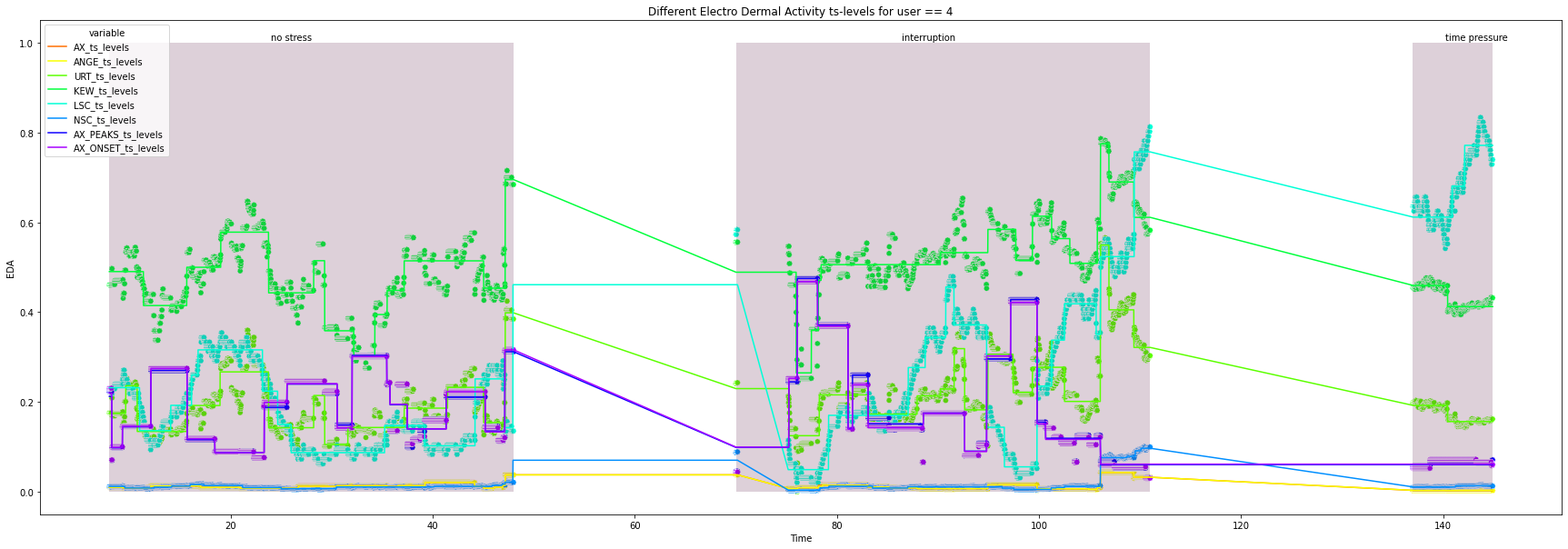
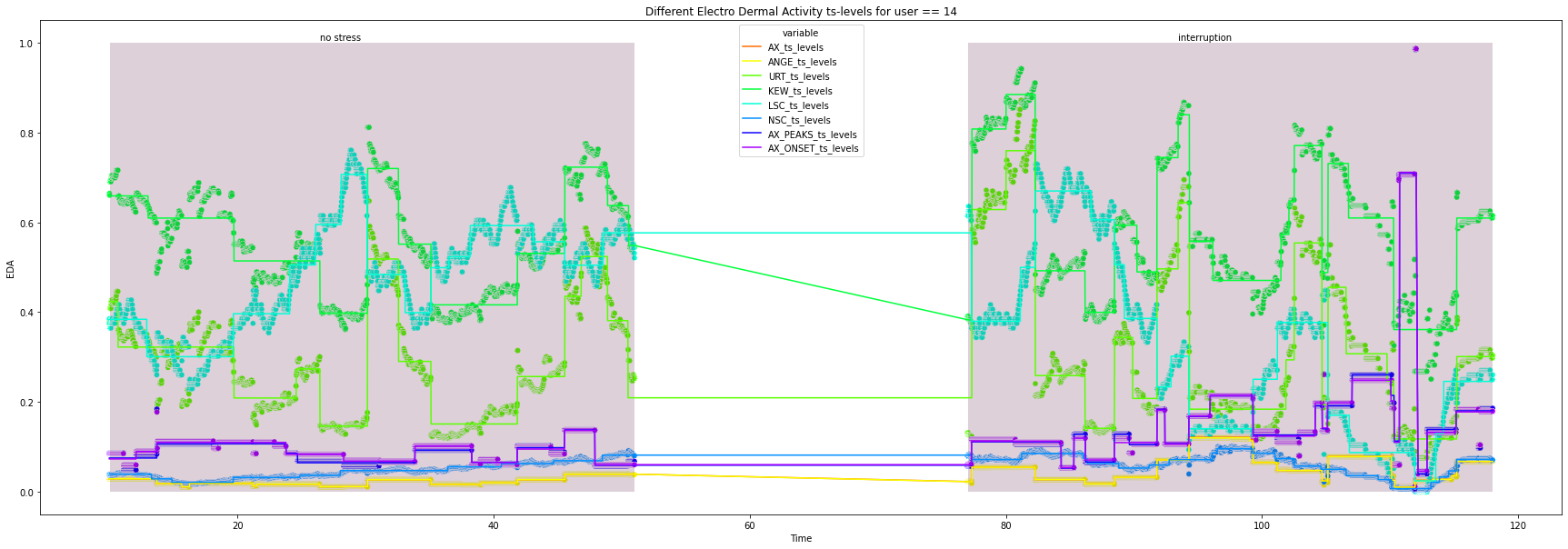
[171]:
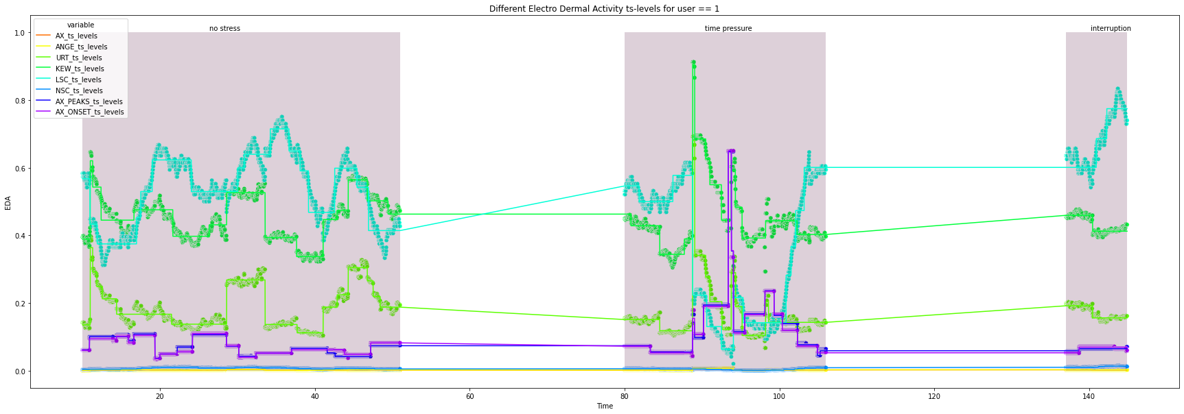
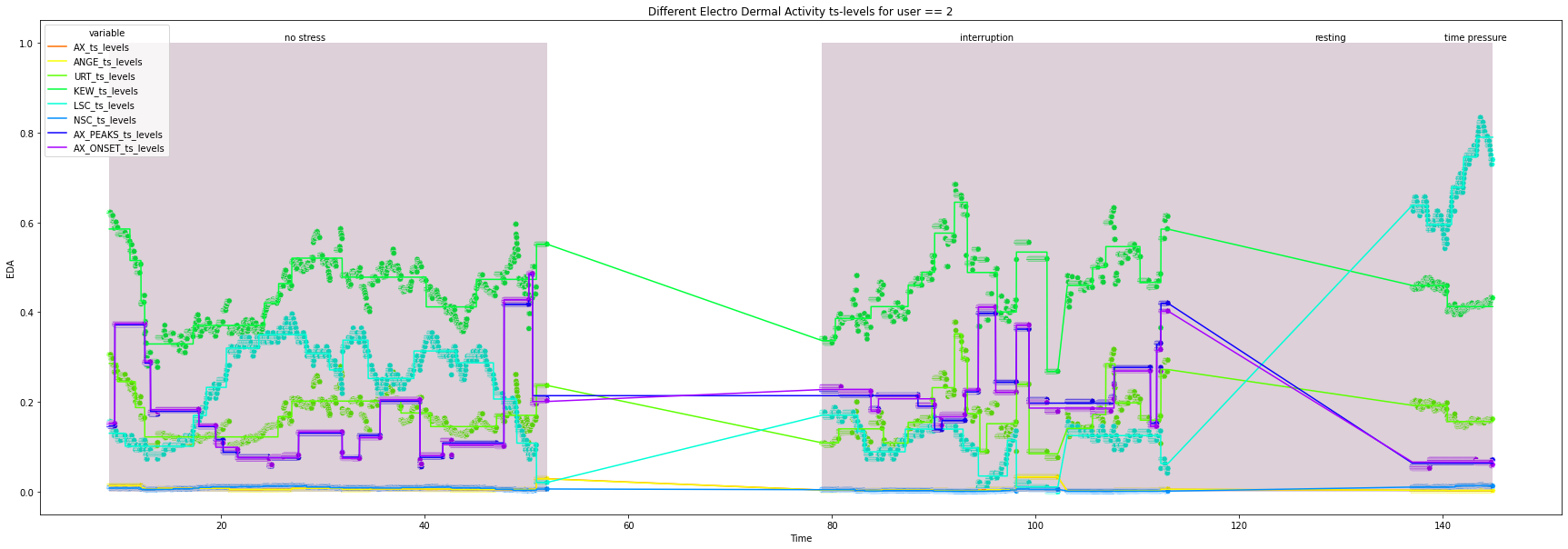
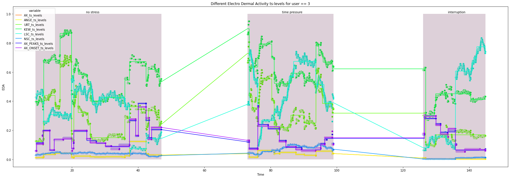
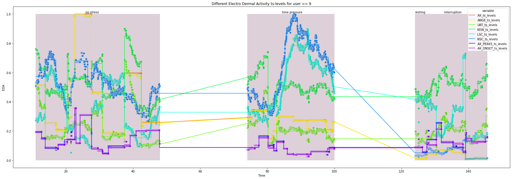
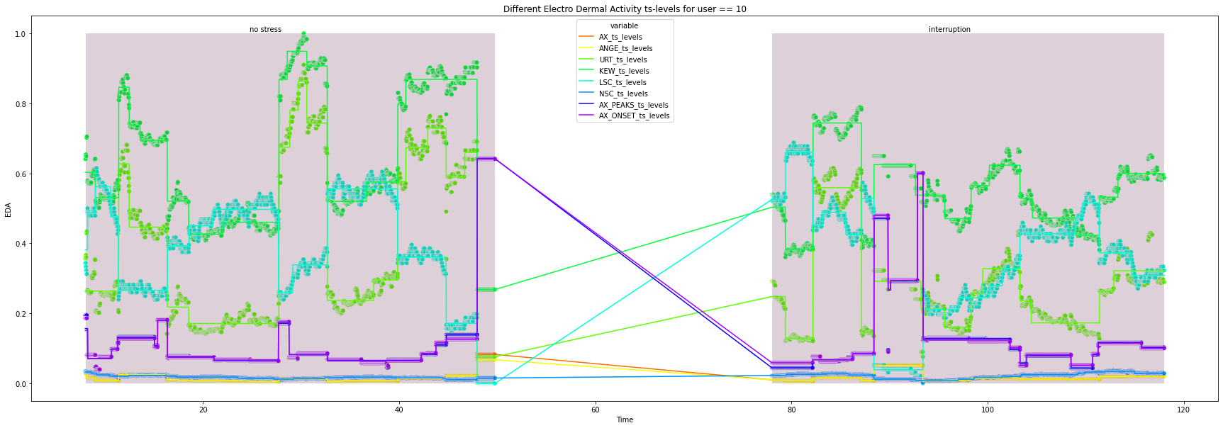
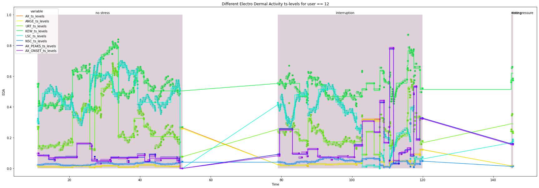
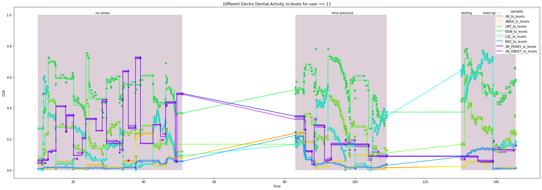
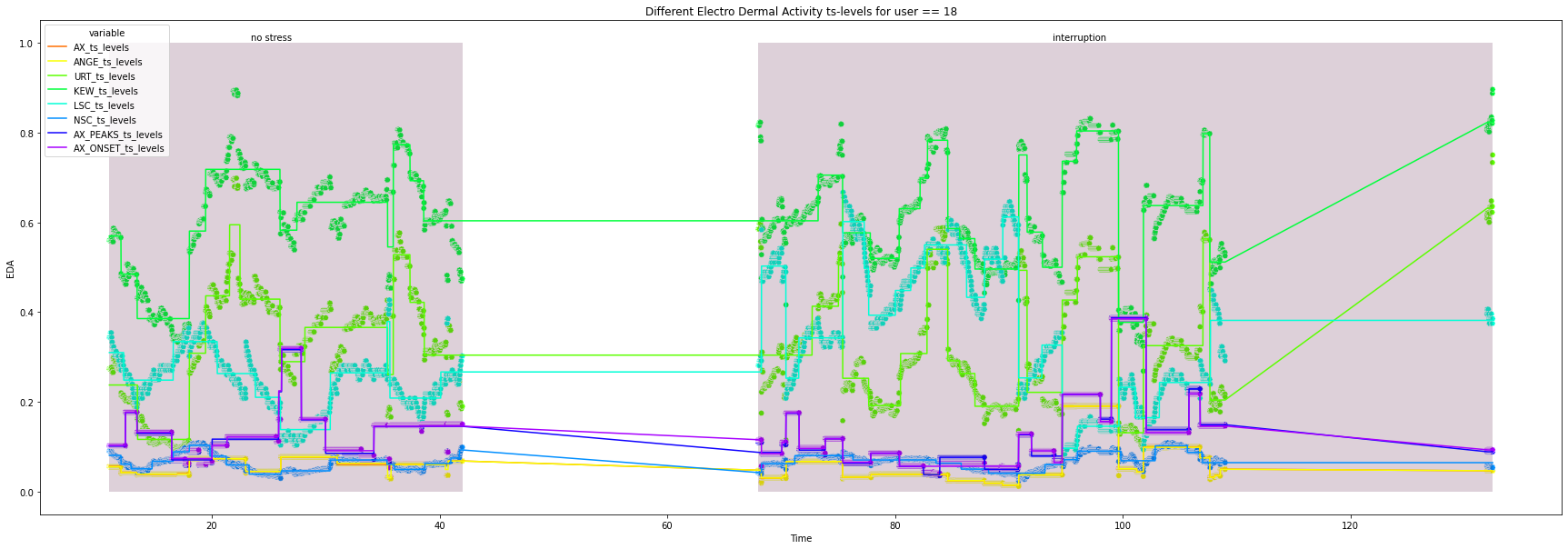
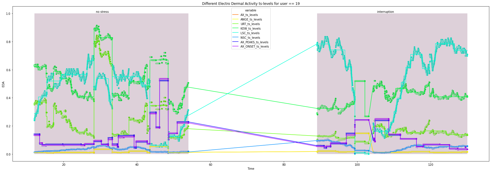
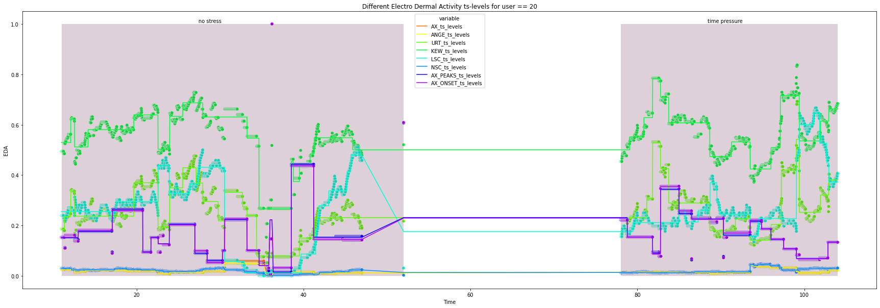
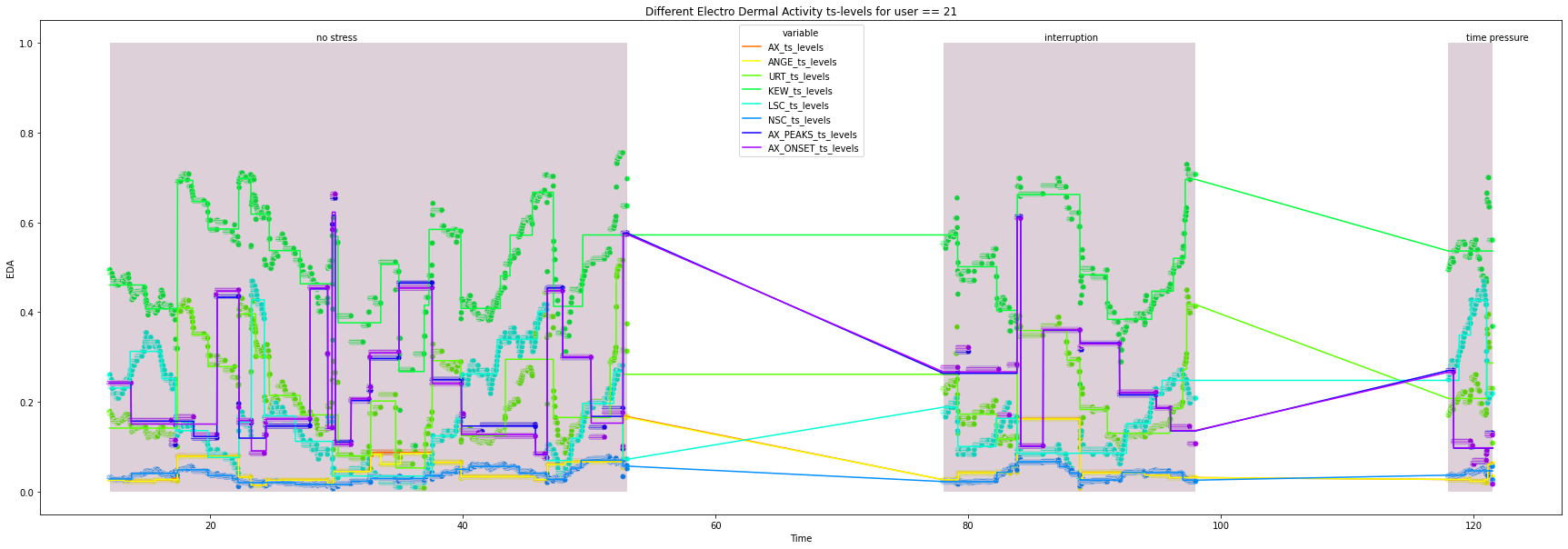
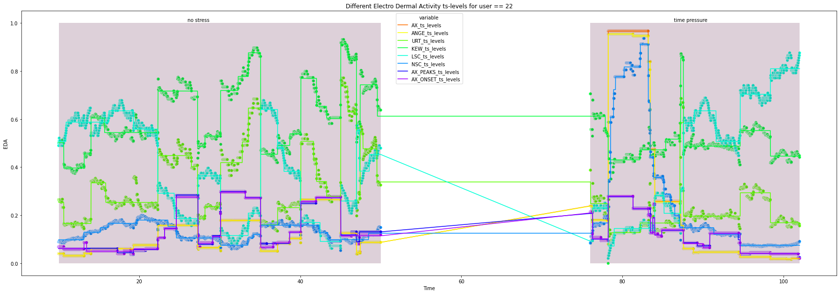
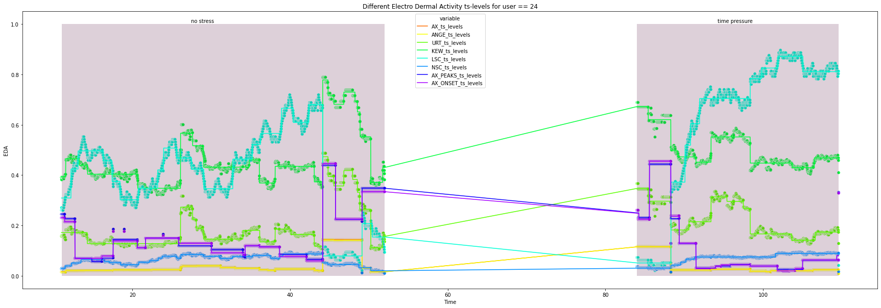
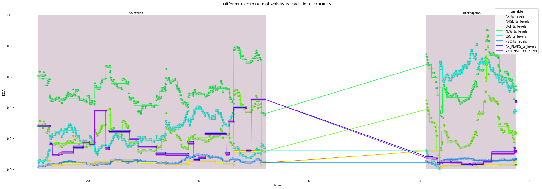
feature_selection = variance_summary[~variance_summary["discard"]].index.tolist()
# feature_selection = swell_eda_features_cols
for user in df["user_id"].unique().tolist():
    print(user)
    ts_df = df.loc[df["user_id"] == user, feature_selection + ["Time", "condition"]]

    all_ts_levels = pd.DataFrame()

    for column in feature_selection:
        ts_levels_df, fig, ax = ts_levels(ts=ts_df[column],
                                      ts_x=None,
                                      criterion="mse",
                                      max_depth=10,
                                      min_samples_leaf=15,
                                      min_samples_split=2,
                                      max_leaf_nodes=30,
                                      plot=False,
                                      equal_spaced=True,
                                      n_x_ticks=10)
        _ = ts_levels_df.set_index("t_steps", inplace=True)
        ts_levels_df.columns = [f"{column[1:]}_{x}" for x in ts_levels_df.columns.tolist()]
        all_ts_levels = pd.concat([all_ts_levels, ts_levels_df], axis=1)

    plot_df = (pd.merge(ts_df["Time"].reset_index(drop=True),
             all_ts_levels,
             left_index=True,
             right_index=True)
           .melt(id_vars="Time"))

    try:
        plt.figure(figsize=(30, 10))
        height=1
        ax = sns.scatterplot(x="Time",
                          y="value",
                          hue="variable",
                          palette="gist_rainbow",
                          data=plot_df[plot_df["variable"].str.contains("original_ts")],
                          legend=False,
                          linestyle='dashed',
                         )
        ax = sns.lineplot(x="Time",
                          y="value",
                          hue="variable",
                          palette="gist_rainbow",
                          data=plot_df[plot_df["variable"].str.contains("ts_levels")],
                         )
        _ = ax.set(xlabel='Time', ylabel='EDA',
                   title=f'Different Electro Dermal Activity ts-levels for user == {user}')

        for condition in ts_df["condition"].unique().tolist():
            x_index = ts_df.loc[ts_df["condition"] == condition, "Time"].index.tolist()[0]+1
            x_co = ts_df.loc[x_index, "Time"]
            width = ts_df.loc[ts_df["condition"] == condition, "Time"].max() - x_co
            _ = ax.add_patch(patches.Rectangle((x_co, 0), width, height, alpha=0.2, facecolor="#581845"))
            _ = plt.text(x=x_co + 0.4*width, y=1.005, s=condition)

        _ = plt.show()
    except:
        print(f"User == {user} plotted with errors")
1
2
3
4
5
6
7
9
10
12
13
14
15
16
17
18
19
20
21
22
User == 22 plotted with errors
24
25
[ ]: